Structural Topic Modeling on the (mostly) Collected Works of Marx and Engels with R
Creative use of text-based data for socialist data science purposes is a main area of interest for my personal research. This is the first in a series of tutorials on using topic models to explore and categorize text-based data. Topic models are machine learning based tools for uncovering the latent thematic structure(s) of a body of text. The aim of this series of documents is both to enhance my own learning in the area and hopefully assist readers interested in using text-based data for socialist purposes get started with using topic models.
We’re going to skip conventional implementations of topic models for now, jumping right away into structural topic models, a greatly improved extension of topic modeling developed specifically for text-based social scientific research. Using STM over conventional TM is only a bit more complicated, yet it is worth learning from the get go as the most useful implementation of topic modeling for the social sciences that currently exists in the R programming language.
This tutorial will be a practical guide to understanding and conducting structural topic modeling in R. In general, my data science education approach is guided by a top-down model of learning, in which explicit and practical knowledge is learned first, which then serves as a foundation for developing implicit knowledge that the practice is based upon.
For the average citizen-data scientist, a good start is aiming to build a robust conceptual understanding of the statistics and modeling algorithms used. Advanced technical knowledge of the complex math and computer science processes that do the work under the hood isn’t necessarily required to make good use of topic models. That goes for data science in general as well. When possible, I’ll be linking to experts that have already laboured to explain aspects of the technical details.
Table of Contents
A brief, practical introduction to topic models for citizen-data scientists
What is topic modeling and how does it work?
Topic models are a sub domain of natural language processing techniques that use probabilistic algorithms developed in computer science to help users discover latent topics contained within unstructured text data. The original authors of the most popular form of topic modeling algorithm based on Latent Dirichlet Allocation describe it as a “generative and probabilistic model of text corpora … where documents are represented as random mixtures over latent topics, where each topic is characterized by a distribution over words”.
It isn’t necessary (at least right away) to know the complicated formulas that make topic modeling work under the surface, but it’s important to have a basic understanding of what a generative model of text does. Models can be generally classified as either discriminative or generative. A discriminative model attempts to use variance in supplied data to make predictions on unknown data; a linear regression is a simple form of this type of model. Generative models, on the other hand, are based on using conditional probability models to generate instances of synthetic data.
So topic modeling with LDA uses statistical inference to actually generate, as synthetic data, topics as probability distributions of terms and documents as distributions of topics. This means that the qualities of the artificial distributions (topics) generated by such models can vary greatly depending on the data and model initialization. This makes preparation, training, evaluation, and interpretation of topic models a bit different from more conventional discriminant models that data science novices might already be familiar with.
- For a clean and concise visual guide to how LDA works as a generative model to produce topics, see here.
- There is an excellent free ebook on inference with LDA using R by Chris Tufts.
- Find a comprehensive and accessible review of best practices in topic modeling written by several experts in this book chapter.
When is it a good idea to use topic modeling?
To reduce the dimensions of large amounts of text data
Topic modeling can be thought of as a form of dimensionality reduction that is specialized for discrete data, which is mostly but not exclusively text data. Large text corpora are ripe targets for the curse of dimensionality. That means topic modeling is an ideal tool to use in any situation where you have a large quantity of text and want to understand the topical content and structure of that text.
Topic modeling reduces the structured data of even massive amounts of text into much more manageable sets of terms and topics. Topic models are also very helpful in facilitating the application of labels of large quantities unstructured text data. In terms of dimension reduction of large text data, you can get a two-for-one deal with topic models. It’s an especially good tool in TMTR situations, where there is just too much text for human beings to read, let alone evaluate and label. As topic modeling expert David Mimno says, “topic models allow us to answer big-picture questions quickly, cheaply, and without human intervention.”
To get an alternative view of just about any set of documents
A topic model can be thought of an an “enhanced” form of reading that allows the user to comprehend all of the topical structure(s) at once within large bodies of texts. It’s basically impossible for a human being, even those with expert familiarity with the texts, to read, process, and analyze a text in such a way, considering the frequency of each term in each document simultaneously, to say nothing of the statistical inference. So topic models provide an alternative way of understanding bodies of text that has been unavailable to human beings until very recently. Obviously, topic modeling is meant as a supplement to, rather than replacement for reading. To the contrary, topic models can often have great potential in the hands of close readers with expert subject matter knowledge.
Raw materials: The data set for this project
In order to begin learning about the theory and practice of text-based data science, we first need some data to use as raw materials. To supply the needed data for the topic modeling project, I wrote a set of functions to scrape the Marxists Internet Archive of all available public domain html text pages, yielding a text data set of over 7100 documents by 43 authors with over 8.5 million rows.
The entire MIA corpus (a fancy way of saying a structured, machine-readable body of texts) is a massive amount of text. Topic models fitted for the entire data set can be huge (10, 20, 30+ Gb) and take a very long time to train depending on the covariate specifications. It’s much more reasonable to begin learning how to use topic models on a smaller subset of the data. In this case, where better to go than back to the original source material: the (almost) collected works of Marx and Engels themselves.
Subsetting the MIA corpus to just the works of Marx and Engels (ME) reduces the size of the data frame from 8.5+ million to a little under 800 thousand rows, a much more manageable amount of text data to experiment with. The ME corpus contains all of their public domain works available from the MIA in html-text format. It includes all texts that are generally considered to be their most important works.
Missing from the ME corpus are the many works taken down due to copyright threats from publisher Lawrence & Wisheart, which includes large portions of their journalistic writings and also personal correspondences. There are also a handful of minor documents that did not play well with the scraping and processing phase of the work. It would be worth restarting the ME topic model again in the future if more works can be added to the data.
Working with tidy text and using a tidy topic modeling workflow
For the most part, the text-as-data course will follow tidy data principles that allow for working with text data using the tidyverse ecosystem of packages. The tidytext package is essential for using tidy methods with text data. If just starting to learn about using text with R, this free book on tidy text mining by Julia Silge, as well as this extensive notebook by Qiushi Yan are invaluable resources.
The essential format of tidy text is one word or token (ex: words, ngrams, sentences, paragraphs, chapters) per row for each document in the. Before the topic modeling workflow can be started, the text needs to be manipulated into tidy format. Having the text in this format, seen below, makes it much easier to turn the text data into a machine-readable form so that calculations can be performed. To see how I prepared the data for this model using tidytext and the tidyverse for cleaning and processing text, see the first part of this tutorial series.
set.seed(1917)
me_corpus_tidy %>%
  slice_sample(prop = .01)
## # A tibble: 7,931 x 4
##    author         year doc                                        word
##    <fct>         <dbl> <chr>                                      <chr>
##  1 Marx           1847 the poverty of philosophy                  germany
##  2 Marx           1863 theories of surplus value                  sell
##  3 Marx           1867 capital, volume i                          roundly
##  4 Marx           1867 capital, volume i                          variable
##  5 Marx           1881 mathematical manuscripts                   differential
##  6 Marx           1894 on the peasantry & precapitalist societies peasants
##  7 Marx & Engels  1894 capital, volume iii                        appropriates
##  8 Engels         1845 condition of working class in england      towns
##  9 Marx           1852 the eighteenth brumaire of louis bonaparte mass
## 10 Marx           1857 the grundrisse                             instrument
## # ... with 7,921 more rows
Readers can find two excellent guides on tidy topic modeling workflows below:
Required data structures
Representing text as a bag-of-words
The basic data structure required for topic modeling is called a “bags of words model”, a method of representing structured text as a vocabulary of unique words or tokens and data on the frequency of occurrence of those terms within documents. Most topic modeling algorithims operate on bag-of-words model text data, so it’s necessary to summarize the text before modeling can begin.
Any tidy tibble of word or token counts is a bag of words model, achieving this data format is the first step to our tidy topic modeling workflow. Start by simply counting the words used in each document, including any other variables you wish to include in the model, in this case the author and year of publication/writing.
me_wordcount <- me_corpus_tidy %>%
  count(doc, author, year, word) %>%
  filter(n > 5)

me_wordcount %>%
  slice_sample(prop = .01)
## # A tibble: 217 x 5
##    doc                                          author         year word       n
##    <chr>                                        <fct>         <dbl> <chr>  <int>
##  1 anti-dühring                                 Engels         1877 valid~    12
##  2 capital, volume iii                          Marx & Engels  1894 varia~    30
##  3 capital, volume i                            Marx           1867 dozen      6
##  4 report to general council of iwma            Marx           1868 class~     6
##  5 theories of surplus value                    Marx           1863 claim      6
##  6 revolution and counter revolution in germany Engels         1852 insur~     8
##  7 theories of surplus value                    Marx           1863 reason    45
##  8 the grundrisse                               Marx           1857 under~    12
##  9 theories of surplus value                    Marx           1863 inver~    15
## 10 capital, volume ii                           Marx & Engels  1885 engla~    11
## # ... with 207 more rows
Inspecting the table, one can see why it’s referred to as a bag of words. The order and structure of the original text are abstracted away exchange for converting the text into quantitative data easily usable by machines. This form of data is comparable to a literal bag of Scrabble tiles, except that the tokens represent quantities of words instead of letters. Despite the lack of order and structure in this way of representing text, topic modeling algorithms are often able to regenerate original documents or held out texts using inference with high levels of success.
Transforming tidy text into a sparse document-term matrix
A minor obstacle to the tidy topic modeling workflow: none of the currently existing TM packages in R can actually take a tidy tibble as input. In order for the words and documents to be used as features in the stm algorithim, the data needs to be converted into some form of document-term matrix, which is a form of sparse matrix of word counts. A sparse matrix is a type of matrix that is largely empty, containing mostly zeroes.
Spare matrices tend to be a rather light-weight way of storing data, since they are mostly empty. It’s a natural data format to use with text because in natural language, a small number of words will be used frequently, while the majority of terms in a vocabulary will be used relatively few times. In this case, we’re going to use tidytext::cast_sparse to turn the tidy word counts into a sparse matrix object.
library(tidytext)
me_sparse <- me_wordcount %>% cast_sparse(doc, word, n)
me_sparse[1:10, 1:2]
## 10 x 2 sparse Matrix of class "dgCMatrix"
##                                                          book bourgeois
## “on proudhon”                                               9        13
## 20th anniversary of the paris commune                       .         .
## address of the central committee to the communist league    .         .
## anti-dühring                                                7        41
## articles in neue rheinische zeitung. revue                  .       227
## bakuninists at work. 1873 spanish revolt                    .         .
## bruno bauer and early christianity                          .         .
## capital, volume i                                          15        37
## capital, volume ii                                         14        10
## capital, volume iii                                        66        19
Many useful functions in topic modeling related R packages, stm included, will only work on document-term or document-feature matrixes, so it’s worth learning how to convert data to and from other formats as well.
Running a structural topic model with model covariates using stm
One of the main improvements of structural topic models with the stm package is the ability to include metadata variables as covariates in the model, opening up many new avenues of analysis in topic modeling. This model uses only the document author and year as metadata, but one can get pretty creative with choosing metadata. Virtually any data that can be connected somehow to the documents in the corpus has metadata potential. Just to name a few possibilities: spatial/geographic data, socioeconomic data, social media or web analytics data, derived scores on the text from something like wordfish as metadata.
In order to include these extra variables in the topic model, a data frame should be constructed, in the same order as the original data, containing the all of the unique combinations of variables associated with each document in the corpus. It’s easy to do by calling dplyr::distinct() on the original data used to cast the sparse matrix.
me_covariates <- distinct(me_wordcount, doc, author, year)
me_covariates %>% head(5)
## # A tibble: 5 x 3
##   doc                                                      author         year
##   <chr>                                                    <fct>         <dbl>
## 1 “on proudhon”                                            Marx           1865
## 2 20th anniversary of the paris commune                    Marx           1871
## 3 address of the central committee to the communist league Marx           1847
## 4 anti-dühring                                             Engels         1877
## 5 articles in neue rheinische zeitung. revue               Marx & Engels  1850
With sparse matrix and co-variate data frame in hand, topic modeling awaits! A structural topic model can be fitted using the stm function. The package authors have written a really detailed paper on how their implementation of topic modeling works. No doubt, when learning to use stm you will be referring back to this paper again and again.
Model co-variates, once supplied with the data argument, are set up using formula notation via the prevalence and content arguments. The former allows the model to account for variance in the prevalence of topics by metadata, while the latter allows for the topic text terms to vary according to the metadata.
The number of topics to include in the model is specified wtih the K argument. Choosing the number of topics is likely the most important input from the user in terms of shaping the outcome of the model. Unfortunately, the “best” number of topics to use cannot be known beforehand, which is why topic modeling is considered an unsupervised form of machine learning.
In this case, we are going with K = 50 topics, using the formula ~ author + year to specify our model covariates, and providing the tibble of metadata to the data argument. The authors of the paper recommend using spectral decomposition as the initialization type for best results. Note that we aren’t setting a seed with set.seed() because according to the package documentation, this form of initialization is deterministic and will produce a stable set of topics with the same data, number of topics, covariates, and paramater tunings.
stm is run with K=0 and spectral initialization, it uses an algorithm created by the authors of this book chapter to determine a number of topics for the user. It doesn’t usually give an ideal number of topics, it does often provide a useful starting point for choosing the number of topics.
library(stm)

me_stm.fit <- stm(
   documents = me_sparse,
   K = 50,
   prevalence = ~ author+year,
   data = me_covariates,
   verbose = TRUE,
   init.type = "Spectral"
 )

# Assign covariates as model-document metadata
me_stm.fit$meta <- me_covariates
After the model has been fitted, it’s important to assign metadata to the fitted model object in order to be able to estimate covariate effects down the road. This can be done by simply assigning the tibble covariates to model.fit$meta. Take a glance at the fitted model to reveal the number of topics, document, terms, and number of model iterations until convergence.
glance(me_stm.fit)
## # A tibble: 1 x 5
##       k  docs terms  iter alpha
##   <int> <int> <int> <int> <dbl>
## 1    50    70  5668    69     1
Use the stm::labelTopics function to print the top words in each topic by several measures. Generally, when assessing the quality of topics take note of the highest probability words associated with each topic. Those terms should be linked by some coherent topical theme that is somehow linked to the text. You’ll also want to make sure that the topics, in addition to being coherent, are also different enough to be useful. FREX is a measure of the frequency and exclusivity of terms, showing the terms that most differentiate the topics. Finally, when looking through the top terms by topics, keep an eye out for the intrusion of seemingly unrelated terms into the topics. Intrusion of off-topic words is often an indicator that the number of topics needs to be adjusted.
labelTopics(me_stm.fit, topics = 1:5)
## Topic 1 Top Words:
##  	 Highest Prob: bourgeoisie, children, manchester, wages, england, time, poor
##  	 FREX: henfrey, pauling, roberts, multitude, maude, disease, filth
##  	 Lift: roberts, alison, damp, lanes, hill, filthy, salford
##  	 Score: manchester, children, operatives, bourgeoisie, wages, report, irish
## Topic 2 Top Words:
##  	 Highest Prob: national, assembly, party, bonaparte, bourgeois, power, parliamentary
##  	 FREX: parliamentary, gentlemen, bonaparte, executive, changarnier, president, bonaparte's
##  	 Lift: electoral, resources, orleans, claremont, elysee, quaestors, dismissal
##  	 Score: bonaparte, assembly, parliamentary, president, gentlemen, party, republic
## Topic 3 Top Words:
##  	 Highest Prob: governments, troops, political, power, struggle, head, june
##  	 FREX: governments, head, june, troops, force, struggle, rule
##  	 Lift: governments, troops, head, june, police, provinces, secret
##  	 Score: governments, troops, june, parliamentary, police, provinces, head
## Topic 4 Top Words:
##  	 Highest Prob: marriage, gens, family, form, gentile, people, stage
##  	 FREX: gens, gentile, gentes, monogamy, barbarism, brothers, sisters
##  	 Lift: gentes, sisters, morgan, consanguinity, kinship, brothers, mother's
##  	 Score: marriage, gens, gentile, gentes, tribe, monogamy, tribes
## Topic 5 Top Words:
##  	 Highest Prob: council, party, civil, war, france, society, political
##  	 FREX: council, party, civil, war, france, indignation, reform
##  	 Lift: council, party, civil, war, france, society, political
##  	 Score: council, party, civil, war, france, society, workers
Choosing the number of topics and evaluating topic model diagnostics
Here’s a catch with topic modeling: there is no rule or statistical test that will simply tell one the “correct” number of topics to use. Topic models are probabilistic and generative models, so a model will produce a different set of topics depending on the initialization of the model.
The distribution, character, and quality of the generated topics are going to change substantially depending on the number of topics chosen and the parameters of the model. In general, lower K will capture less variance in the data, resulting in broader topics with more common shared terms. On the other hand, specifying more topics with a higher K captures more variance in the data, producing more fine grain, focused topics.
According to the package authors, it’s generally preferable to have more, rather than fewer topics. In general, higher K will produce better topics, but past a certain point, the coherence of the topics can quickly breakdown as the algorithm “overlearns” the data. Seeing many topics that overlap too much to be useful is another sign that K might be too high. However, having K too low can also produce overlapping, overly-broad topics by failing to capture enough variation in the text. So there is quite a bit of nuance required in selecting a suitable number of topics.
In general, the more text data that a corpus contains, the higher K will need to be to produce enough topics to unveil the structure of the data. At the same time, larger corpora also have a higher threshold for increasing K before the topic boundaries begin to turn mushy.
Running and comparing many models
Different algorithms for automatically choosing K have been proposed, but ultimately it will depend on the user’s subjective assessment of the coherence and quality of the topics and how they relate to the original texts. It also depends, of course, on what the actual purpose of running the topic model is in the first place.
Looking at a model in isolation, it can be hard to judge how to improve the model by adjusting the number of topics. The solution is to run many models with different numbers of topics and compare the results. The vantage point provided by viewing the models in relation to each other makes it much easier to narrow down a range of K values to begin experimenting with.
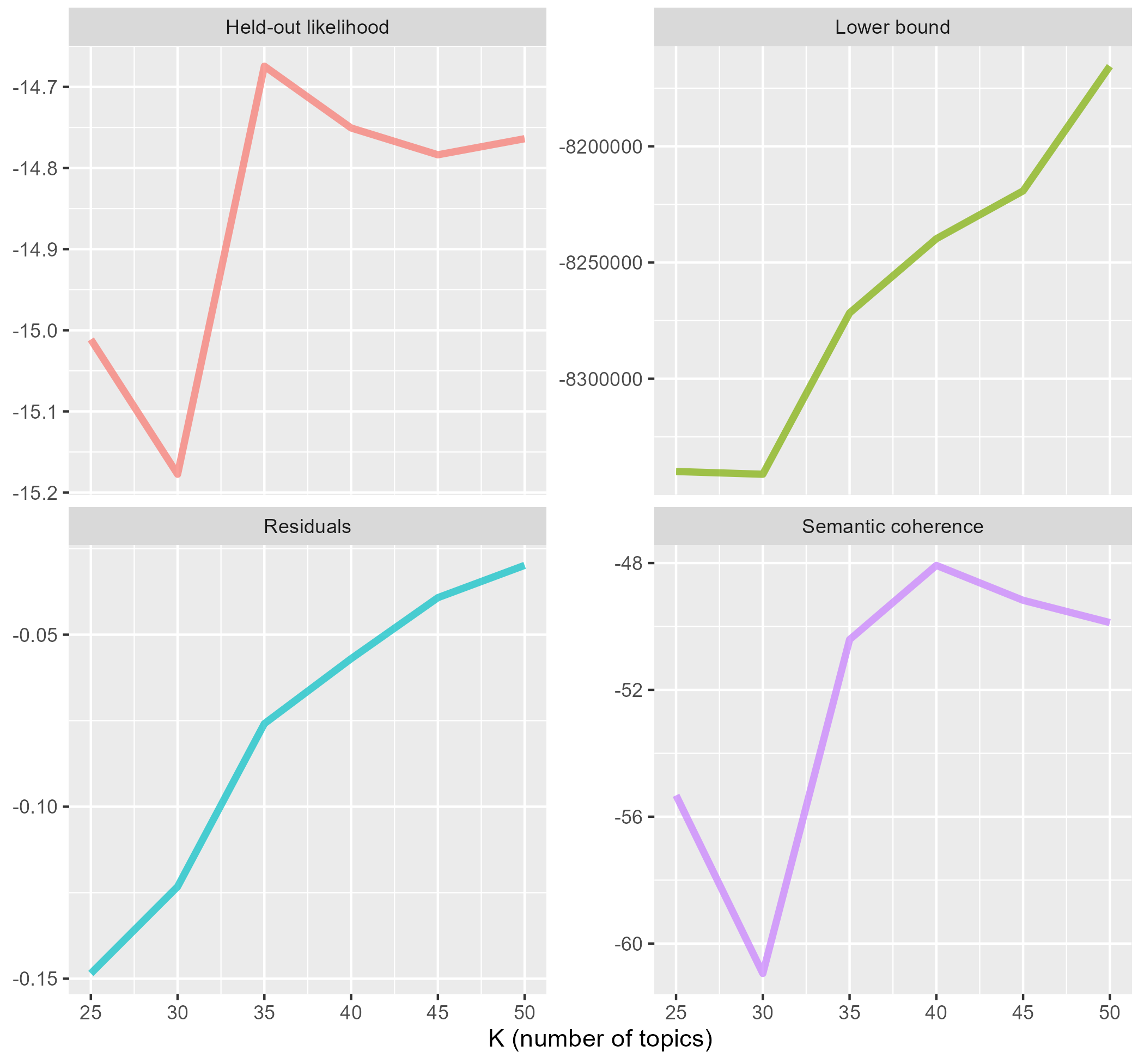
Below is a method for running and comparing many models using a sparse matrix provided in this very useful tutorial by Julia Silge.
library(furrr)
plan(multiprocess)

many_models <- data_frame(K = c(25, 30, 35, 40, 45, 50)) %>%
  mutate(topic_model = future_map(K, ~stm(mia_sparse, K = .,
                                          verbose = FALSE)))


heldout <- make.heldout(mia_sparse)

k_result <- many_models %>%
  mutate(exclusivity = map(topic_model, exclusivity),
         semantic_coherence = map(topic_model, semanticCoherence, mia_sparse),
         eval_heldout = map(topic_model, eval.heldout, heldout$missing),
         residual = map(topic_model, checkResiduals, mia_sparse),
         bound =  map_dbl(topic_model, function(x) max(x$convergence$bound)),
         lfact = map_dbl(topic_model, function(x) lfactorial(x$settings$dim$K)),
         lbound = bound + lfact,
         iterations = map_dbl(topic_model, function(x) length(x$convergence$bound)))
 If you are working with documents in one of the other object classes for holding a DFM instead, it’s also possible to use the
 searchK() function provided by the stm package. The upside of this method is that it requires far less code; the model diagnostics are automatically calculated and retrieved and that the plot can be recreated simply by calling plot() on the output of searchK. The main downside of this method is that it isn’t easily possible to retrieve the model diagnostics in a tidy tibble as above for easy manipulation with the tidyverse and more advanced plotting options with ggplot2.
# Convert the sparse matrix
me_corpus <- asSTMCorpus(documents = me_sparse,
                         data = me_covariates)

me_searchK <- searchK(me_corpus$documents,
                      me_corpus$vocab,
                      K = c(25),
                      data = me_corpus$data,
                      init.type = "Spectral",
                      prevalence = ~ author + year
                  )

plot(me_searchK)
Typically, the aim in selecting a model here is to minimize residuals while maximizing semantic coherence. Consider models with higher held-out values as well, indicating models that perform better in using their generated topics to reconstruct the held-out texts by calling stm::make.heldout() on the sparse matrix.
Settling on a topic model is usually an iterative process of running models with different numbers of topics and parameters, then exploring and validating the constructed topics. The diagnostic plot above initially suggested starting with a range of 35 to 40 topics, but after many iterations of running models and doing detailed evaluation of topics at different K values, 50 topics was selected as having the best distribution of quality topics across the 70 documents in the corpus.
The delicate dance between semantic coherence and exclusivity
Semantic coherence is a measure of co-occurrence of terms within topics, with more co-occurrence closer to zero. In general, semantic coherence tends to track well with expert judgement of topics as meaningful and useful. This comparison won’t tell you the “correct” number of topics to use, but it will give a very solid range of K to begin experimenting with.
Unfortunately, one cannot see a high semantic coherence score and assume a high quality, usable topic. A small number of topics with mostly common words could be high in semantic coherence, yet not capture enough variance in the data to be meaningful or useful. The authors of the stm package have created a function to measure topic exclusivity based on the FREX values of it’s associated terms. The closer to 100, the more exclusive the terms are to a particular topic.
The stm package features easy to use functions for computing both semantic coherence and exclusivity.
excl <- exclusivity(me_stm.fit)
semcoh <- semanticCoherence(me_stm.fit, me_sparse)
diag_df <- tibble(excl, semcoh, topic = factor(1:50)) %>% left_join(topic_labels)
diag_df
## # A tibble: 50 x 5
##     excl semcoh topic category             color
##    <dbl>  <dbl> <fct> <chr>                <chr>
##  1  8.88  -22.8 1     Sociology            #8f1f3f
##  2  9.70  -64.2 2     Politics             #de860b
##  3  9.98  -62.4 3     Politics             #de860b
##  4  9.57 -110.  4     Anthropology/History #d4ae0b
##  5  9.99  -52.7 5     Politics             #de860b
##  6  9.99  -45.0 6     Sociology            #8f1f3f
##  7  9.86  -85.4 7     Sociology            #8f1f3f
##  8  9.97  -57.6 8     Anthropology/History #d4ae0b
##  9  9.46  -81.1 9     Philosophy           #c73200
## 10  9.99  -59.5 10    Sociology            #8f1f3f
## # ... with 40 more rows
Each topic can be seen as trading off between the co-occurrence and exclusivity of the terms that comprise it. A high quality topic will have typically have both coherence and exclusivity somewhere on the moderate to high range. A good set of topics will have a relatively balanced distribution of exclusivity and coherence across each topic.
Once you have settled on a model K it is worth taking a closer look at the distribution of exclusivity and coherence across each topic. Have a closer look into any topics that appear out of place on the exclusivity vs. coherence topic scatter plot. Having a low score on either doesn’t necessarily indicate a low quality topic.
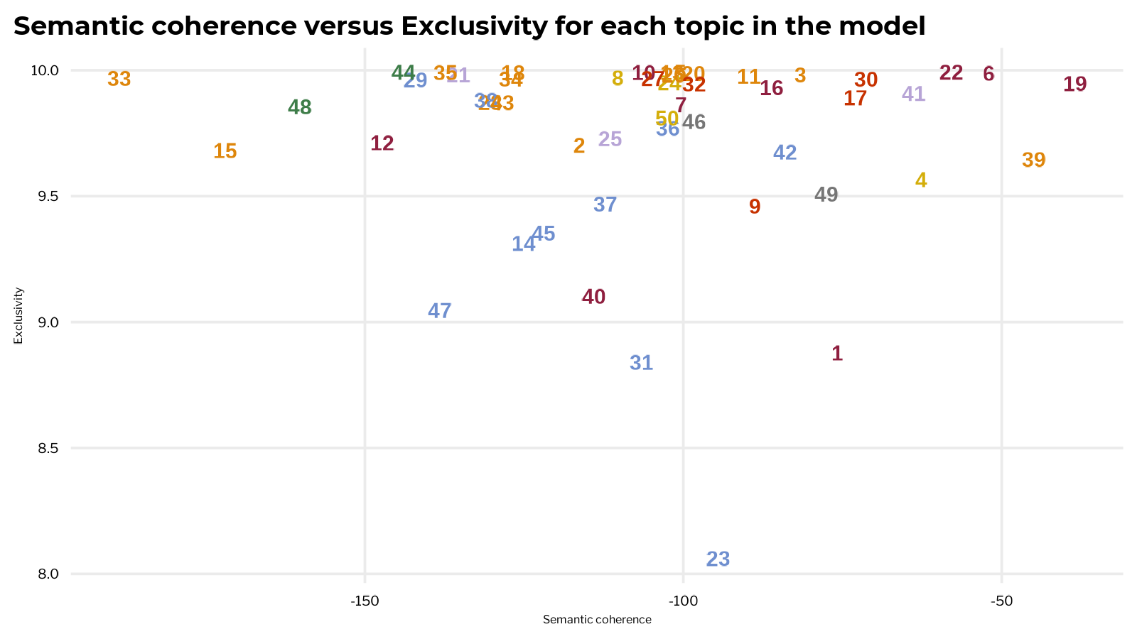
Topic 33
Despite having the lowest semantic coherence score in the model, topic 33 does appear to have a consistent theme, with terms related (1) to general terms related to political science and (2) to discussing Swiss politics specifically.
It’s possible that there are two latent topics here, one on politics in general, one on politics in a specific time/place, that could split apart with more topics or different model initialization. However, it’s also possible that their writings on Swiss politics were more important to their political works than one would initially assume. Marx did spend several formative years studying philosophy in Switzerland after all.
labelTopics(me_stm.fit, topics = 33)
## Topic 33 Top Words:
##  	 Highest Prob: congress, conference, sections, alliance, rules, section, committee
##  	 FREX: conference, geneva, federation, rules, sections, basel, fonds
##  	 Lift: council's, conference, basel, fonds, geneva, federation, malon
##  	 Score: conference, congress, geneva, alliance, federal, sections, federation
Topics 23 and 47
Several the topics on political economy in the Marx/Engels corpus (topics 23, 47) are a bit lower on exclusivity because they share many common terms. But these topics remain coherent and useful because they clearly discuss different aspects of a related subject: labour and the production process (23) and exchange, circulation, and the realization of capital (47). Given how constantly Marx and Engels talk about labour throughout their works, the especially low exclusivity of 23 in the model seems to check out.
labelTopics(me_stm.fit, topics = c(23, 47))
## Topic 23 Top Words:
##  	 Highest Prob: labour, production, capital, form, means, hours, time
##  	 FREX: workpeople, whilst, spindle, coat, productiveness, requisite, workman
##  	 Lift: apes, whilst, spindle, pm, statute, vanishes, workpeople
##  	 Score: labour, hours, labourer, labourers, linen, capitalist, capital
## Topic 47 Top Words:
##  	 Highest Prob: labour, capital, production, time, exchange, money, circulation
##  	 FREX: thalers, posited, objectified, posits, realization, presupposed, instrument
##  	 Lift: realize, laboring, posits, posit, positing, stp, fixated
##  	 Score: capital, labour, thalers, circulation, surplus, posited, exchange
Working with topic model output using the tidyverse
The tidytext package adds methods to the broom::tidy() function for tidying up the output of topic models into tibbles. One of the best parts of using a tidy approach to modeling in R is that it allows use of the tidyverse ecosystem of packages on model output. That opens up all sorts of possibilities for manipulating, visualizing, and computing on model output.
Using tidy with matrix = "beta" will grab the model’s beta matrix and place it in a tidy tibble. Beta gives the topic-term expected probability for every term in the vocabulary for each topic. Recall that topic models treat each topic as a distribution of each term in the vocabulary. To measure how strongly terms are associated to topics, use beta. Note the absence of metadata in the beta matrix, since that data is attached to documents and not the terms that appear in them.
# per-term per-topic probability - millions of rows before filtering!
stm_beta <- tidy(me_stm.fit,
                    matrix = "beta",
                    document_names = me_stm.fit$meta$doc) %>%
  group_by(topic) %>%
  slice_max(beta, n = 5000, with_ties = FALSE) %>%
  arrange(topic, desc(beta), .by_group = TRUE) %>%
  mutate(topic = as_factor(topic))

stm_beta %>%
  arrange(-beta) %>%
  head()
## # A tibble: 6 x 3
## # Groups:   topic [5]
##   topic term         beta
##   <fct> <chr>       <dbl>
## 1 6     classes     0.994
## 2 3     governments 0.980
## 3 10    social      0.809
## 4 22    property    0.503
## 5 22    workers     0.494
## 6 5     council     0.493
Calling tidy with matrix = "gamma" will turn the gamma matrix into a tibble. Topic models treat each document as a mixture of certain topics. Gamma is a measure of the expected topic-document probability for each document. In other words, use gamma to find out which topics each document is composed of and the strength of those topic-document relationships.
# per-document per-topic (also called theta)
stm_gamma <- tidy(me_stm.fit,
                          matrix = "gamma",
                          document_names = me_stm.fit$meta$doc) %>%
  right_join(me_covariates, by = c('document'= 'doc')) %>%
  group_by(topic) %>%
  arrange(topic, desc(gamma)) %>%
  mutate(topic = as_factor(topic))

stm_gamma %>%
  arrange(-gamma) %>%
  head()
## # A tibble: 6 x 5
## # Groups:   topic [6]
##   document                                        topic gamma author  year
##   <chr>                                           <fct> <dbl> <fct>  <dbl>
## 1 on the history of early christianity            27    0.999 Engels  1894
## 2 introduction to critique of philosophy of right 30    0.999 Marx    1843
## 3 mountain warfare in the past and present        25    0.999 Engels  1857
## 4 the dialectics of nature                        49    0.998 Engels  1883
## 5 on afghanistan                                  21    0.998 Engels  1857
## 6 mathematical manuscripts                        46    0.996 Marx    1881
The tidy gamma tibble also contains the model metadata, which is provided at the document level. Use the gamma matrix to pry the metadata out of the model for further use. For this model, we are only using author and year as metadata. To connect the model terms in each topic to the model covariates, the beta and gamma tibbles need to be joined in some manner.
To combine model terms with topics, start by grouping by topic, selecting the top 3 terms by term-topic probability (beta) for each topic in the model, then summarizing, pasting, and unnesting to collapse the top terms by topic into a single vector.
# Top 4 terms for each topic by beta for labeling
me_beta_topterms <- me_tidy_beta %>%
  group_by(topic) %>%
  slice_max(beta, n = 3) %>%
  select(topic, term, beta) %>%
  summarise(terms = list(term)) %>%
  mutate(top_terms = map(terms, paste, collapse = ", "), topic = as_factor(topic)) %>%
  unnest(cols = top_terms) %>%
  select(topic, top_terms)
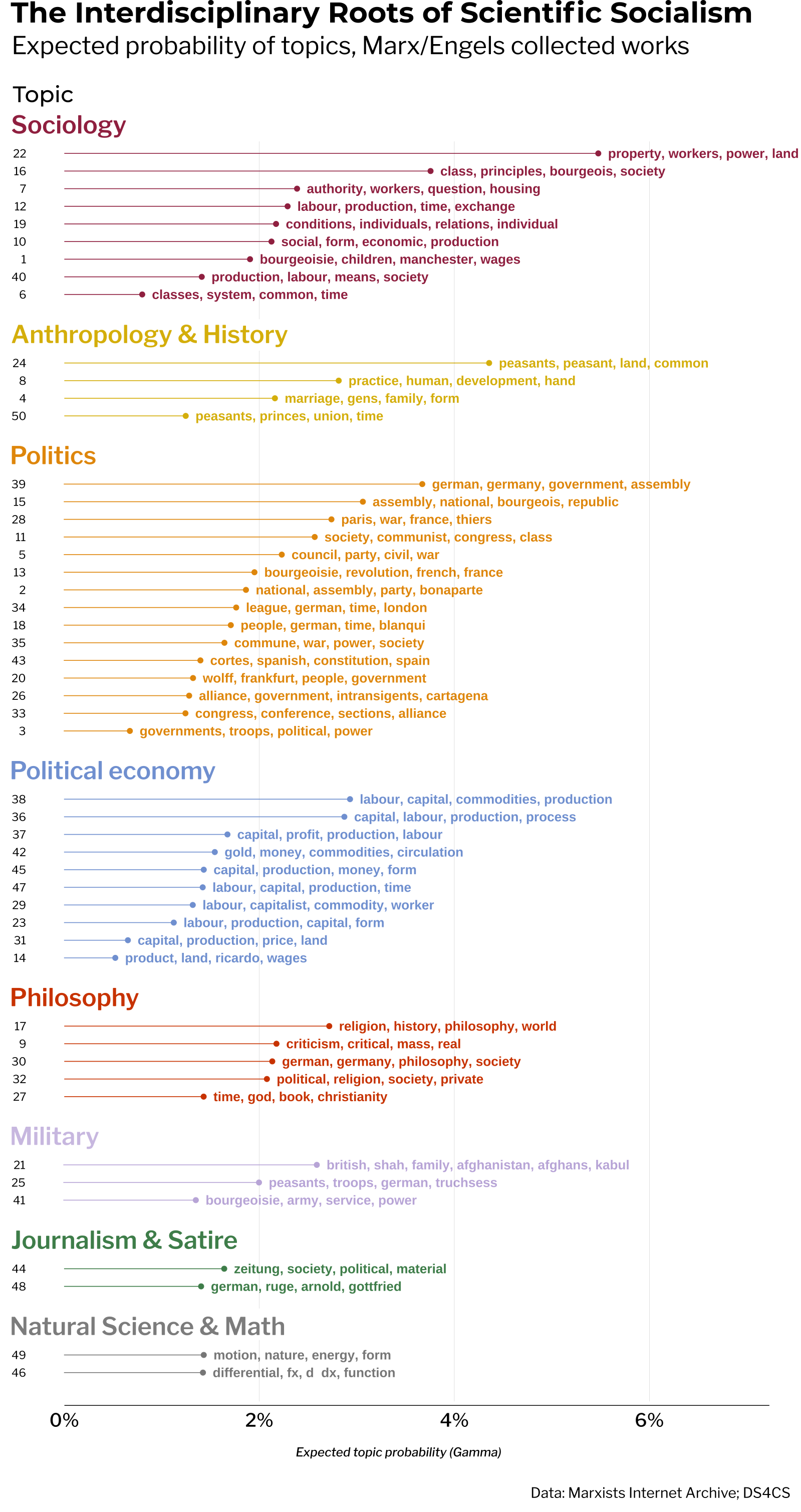
From there, the average gamma per topic is calculated, giving a measure of how strongly each topic is associated with the entire corpus of documents. Then the average gamma tibble is joined with the top terms by topic so that the combined terms can be used as labels in the chart below.
# Combine top terms with average topic gamma
me_tidy_bg <- me_tidy_gamma %>%
  group_by(topic) %>%
  summarise(gamma = mean(gamma, na.rm = TRUE)) %>%
  arrange(-gamma) %>%
  left_join(me_beta_topterms) %>%
  mutate(topic = reorder(topic, gamma))

me_tidy_bg %>% head(5)
## # A tibble: 5 x 3
##   topic  gamma top_terms
##   <fct>  <dbl> <chr>
## 1 22    0.0548 property, workers, power
## 2 24    0.0436 peasants, peasant, land
## 3 16    0.0376 class, principles, bourgeois
## 4 39    0.0368 german, germany, government
## 5 15    0.0307 assembly, national, bourgeois
Exploring the structural topic model of the Marx/Engels corpus
After assessing the model diagnostics, it’s time to start building a deeper understanding of the topic model. A good way to start is by plotting the distribution of average topic gamma and the top terms from per topic from me_tidy_bg to gain a good overview of the topic structure of the model.
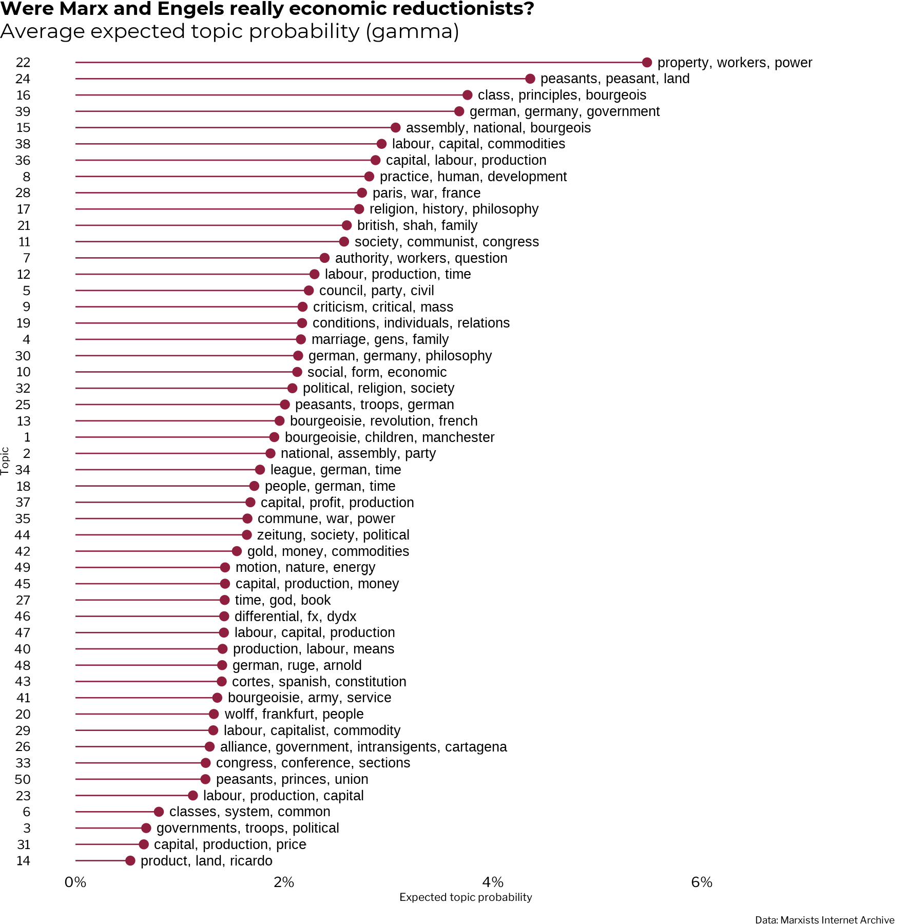
Scanning the order of topics and the top terms of each, it’s immediately apparent that Marx and Engels wrote about a great diversity of subjects. This view of the model suggests that, in written form at least, the scientific socialist method draws upon many aspects of social sciences and humanities at large. It’s hard to imagine how an analysis of this kind could be recreated easily using raw text counts or dictionary based methods.
How topic models help humans categorize large amounts of data
One of the main purposes of topic models is to assist human beings in labeling and categorizing, thereby imposing structure, on large amounts of unstructured text-based data. It’s interesting and informative to look over the distribution of 50 topics above, but even 50 topics is quite a few features to work with for many purposes. A corpus with too much text to read can often produce too many topics to use individually. Initial experimental topic model runs on the entire MIA corpus of over 7000 documents produced well over 200 topics. Even larger models, containing hundreds of thousands or even millions of documents, could produce topic sets of astounding size.
In order to make working with many topics easier, it’s common to follow up topic modeling with further labeling or categorization of topics. Grouping topics and their associated terms according to a categorical label variable introduces structure to the set of topics by reducing the number of dimensions in the data.
When facing an unworkable number of topics, it’s common to employ further machine learning algorithms to do semi-supervised or automatic classification of topics. In this case, due to the small number of topics, the good quality and coherence of the topics, and my existing domain knowledge regarding Marxism and Marx’s work specifically, I chose to label the topics manually.
Substantial creative license exists regarding the choice of category labels. What makes a set of good and useful labels? It’s hard to say, since it depends on the user’s domain knowledge, the qualities of the texts, the purpose for the research and specifically the reason for applying labels to the data.
For the ME topic model, I went with manually categorizing the topics into broader disciplinary subject areas. Looking closer into the terms and documents associated with the topics, it was relatively simple to place each topic into a category denoting a major subject area in the social sciences or humanities. There certainly could be some debate over, for instance, where sociology ends and political economy or philosophy begins. Often, teams of coders will categorize topics and use objective metrics to measure the inter-rater reliability of the labels.
A note on the importance of domain knowledge in data science
Domain knowledge is exceptionally important for novice data scientists. It takes years of study and practice to build expertise in things like mathematics, statistics, machine learning, and software engineering. But you’re probably already very knowledgeable about some things! Creative use of data can go a long way when leveraged with some domain knowledge.
Due to my existing domain knowledge, I felt confident that I could perform the topic categorization on my own. In the course of studying political science and sociology, I have had the opportunity to read deeply within the social sciences and Marxism specifically. I’ve read all of the major works of Marx and Engels multiple times and have done much secondary reading that situates their writing in proper historical and methodological context.
Someone lacking that domain knowledge would no doubt find manually applying labels to topics in this manner much more challenging. For those users, there could be value in applying further unsupervised techniques like hierarchical clustering to suggest at possible groupings even in smaller topic sets. However, it’s likely that a user with a good base of knowledge in the social sciences, even without great familiarity with Marxism or the writings of Marx/Engels, could probably reach similar conclusions by doing a small amount of contextual research as needed.
Unveiling the inherently interdisciplinary nature of Marxism with topic modeling
This is the point where, in my humble opinion, the real potential of topic modeling plus data categorization is demonstrated. By applying labels to topics according to broad disciplinary categories, the factor topic with 50 levels is re-coded into category, a factor with only 8 levels: anthropology/history, journalism/satire, philosophy, politics, political economy, military, sociology, and science/math.
When coding a small to moderate number of topics manually, I like to use a tribble with list-columns for the associated topics of each disciplinary subject area. Using double unnest on the list-column produces a tidy tibble of topic-category labels that can be joined to the tidy model output.
topic_labels <- tribble(
  ~topic, ~category, ~color,
  list(4, 8, 24, 50), "Anthropology/History", "#d4ae0b",
  list(44, 48), "Journalism/Satire", "#3E7D49",
  list(9, 17, 27, 30, 32), "Philosophy", "#c73200",
  list(2, 3, 5, 11, 13, 15, 18, 20, 26, 28, 33, 34, 35, 39, 43), "Politics", "#de860b",
  list(14, 23, 29, 31, 36, 37, 38, 42, 45, 47), "Political Economy", "#6F8FCF",
  list(21, 25, 41), "Military", "#b7a4d6",
  list(1, 6, 7, 10, 12, 16, 19, 22, 40), "Sociology", "#8f1f3f",
  list(46, 49), "Science/Math", "#767676") %>%
  unnest(topic) %>%
  unnest(topic) %>%
  mutate(topic = factor(topic))

topic_labels
## # A tibble: 50 x 3
##    topic category             color
##    <fct> <chr>                <chr>
##  1 4     Anthropology/History #d4ae0b
##  2 8     Anthropology/History #d4ae0b
##  3 24    Anthropology/History #d4ae0b
##  4 50    Anthropology/History #d4ae0b
##  5 44    Journalism/Satire    #3E7D49
##  6 48    Journalism/Satire    #3E7D49
##  7 9     Philosophy           #c73200
##  8 17    Philosophy           #c73200
##  9 27    Philosophy           #c73200
## 10 30    Philosophy           #c73200
## # ... with 40 more rows
The infographic below shows the exact same data as the previous chart, the distribution of topics by average document-topic gamma and the top terms for each topic. The only difference is that the data has been faceted and coloured by the category of discipline the topic falls under.
Such a small change has a great impact: revealing the inherently interdisciplinary nature of Marxism, as found in the original source material produced by Marx and Engels themselves. It conveys how the Marxist method of historical materialism, as developed by the Marx and Engels themselves, pushes against one-sided interpretations of complex social phenomena. Their project of scientific socialism necessitated an interdisciplinary, holistic approach to grasp the complex, multifaceted reality of capitalism. It was necessary to develop such a thorough understanding of capitalism in order to create a many-sided scientific formulation of it’s negation and replacement by a superior mode of production, e.g. Marxism.
These findings fly in the face of the still popular (especially in liberal humanities circles and certain sectors of chronically-online quasi-left discourse) one-sided caricature of Marxism as tainted by “economic” or “class” reductionism found in the works of Marx/Engels and leading all the the way to Marxism today.
Topic modeling reveals something about the intellectual method of Marx and Engels and by extension of Marxism at large that usually not apparent to either shallow critics of or many newcomers to Marxism: namely the holistic, flexible, and multi-faceted nature of the historical materialist method. These historically neglected aspects of Marx’s project has been emphasized in recent years by a small number of Marx scholars in recent years, such as Kevin B. Anderson or Marcello Musto.
Of course, topic modeling is no replacement for good old fashioned deep-reading. If one is interested in being a Marxist, one should attempt to read and digest at least the major works of Marx and Engels. It is also certainly not a substitute for reading expert scholars on the topic like those cited above. I can imagine, for example, that there could be value in incorporating the information and graphics produced with this topic model into an introductory reading guide to the Marx/Engels body of work for beginner Marxists.
Evaluating the quality of user applied topic labels with dimension reduction
Visualizing topic-document-label (gamma) relationships
At this point, we’ve already evaluated the individual topics and the distribution of topics as a whole in a number of ways, including computed metrics (semantic coherence, exclusivity) and subjective judgement in terms of thematic coherence and usefulness. It’s also sound practice to evaluate the quality of the categorical topic labels, since they are often going to used as the main unit of analysis and reporting in further work.
It’s possible to evaluate how the categorical topic labels are related to the terms, topics, and documents in the model using dimension reduction to get a higher level view of the structure of the data. To obtain a measure of how the document and their associated topics are related to the manually applied category labels, calculate the average gamma of the topics related to each document, grouped by category, then pivot the data into wide format. After that, transform the tibble into a matrix so that it can be fed into the dimension reduction algorithms.
# Summarize the data by average gamma, then pivot the category column into wide format
me_gamma_wide <- me_tidy_gamma %>%
  select(document, category, topic, gamma) %>%
  group_by(category, document) %>%
  summarise(gamma = mean(gamma)) %>%
  pivot_wider(id_col = document, names_from = category, values_from = gamma)

# Convert the wide gamma tibble to a matrix
gamma_matrix <- as.matrix.data.frame(me_gamma_wide[,2:8], rownames.force = TRUE)
rownames(gamma_matrix) <- unique(me_gamma_wide$document)

gamma_matrix[1:5, 1:2]
##                                                          Anthropology/History
## “on proudhon”                                                    1.398080e-04
## 20th anniversary of the paris commune                            8.708505e-05
## address of the central committee to the communist league         2.832201e-04
## anti-dühring                                                     4.664125e-06
## articles in neue rheinische zeitung. revue                       7.170735e-02
##                                                          Journalism/Satire
## “on proudhon”                                                 1.488253e-07
## 20th anniversary of the paris commune                         1.557863e-09
## address of the central committee to the communist league      9.395111e-06
## anti-dühring                                                  1.728004e-11
## articles in neue rheinische zeitung. revue                    2.747868e-10
The result is a matrix where rows represent documents in the corpus and columns encode the average document-topic probability (gamma) of the topics that comprise each category. First, reduce the gamma-category matrix using principal component analysis via the base R prcomp function. After that, the principal components are further reduced and projected in two-dimensions using an Uniform Manifold Approximation and Projection (UMAP) algorithm with the umap::umap() function. For more on how to fine tune the parameters of a UMAP algorithm, check out this tutorial.
library(umap)
library(RSpectra)

## Conduct PCA
me_gamma.pca <- prcomp(gamma_matrix)

## Followed by UMAP
me_gamma_umap <- umap(me_gamma.pca$x,
                      n_neighbors = 4,
                      n_epochs = 500,
                      spread = 6,
                      min_dist = .7,
                      seed = 1876
                      )

## Predict UMAP results
me_gamma_umap.pred <- predict(me_gamma_umap, me_gamma.pca$x)
me_gamma_umap.pred %>% head(5)
##                                                               [,1]        [,2]
## “on proudhon”                                            -1.431028   8.4224398
## 20th anniversary of the paris commune                     4.360857 -12.9230463
## address of the central committee to the communist league  3.103039  17.1232316
## anti-dühring                                             -1.659779  19.4914560
## articles in neue rheinische zeitung. revue                5.779645   0.7873275
From there, a little bit of data wrangling is needed to get the UMAP output into a tidy form that agrees with ggplot2. Using predict on the umap output returns the UMAP dimension data for each document in the data. The main category label associated with each document is decided by averaging gamma for each topic in the document according to category, then selecting the category with the highest average gamma. Finally, the umap output is converted into a tibble and joined with the category and colour labels in doc_cats.
cat_colors <- distinct(topic_labels, category, color)

doc_cats <- me_tidy_gamma %>%
  group_by(document, category) %>%
  summarise(gamma = mean(gamma)) %>%
  slice_max(gamma, n = 1, with_ties = FALSE) %>%
  left_join(cat_colors) %>%
  select(document, category, color)

gamma_umap_df <- me_gamma_umap.pred %>%
  as_tibble(rownames = "document") %>%
  rename(umap1 = V1, umap2 = V2) %>%
  left_join(doc_cats, by = "document") %>%
  select(category, document, color, umap1, umap2)

gamma_umap_df %>% head()
## # A tibble: 6 x 5
##   category             document                             color  umap1   umap2
##   <chr>                <chr>                                <chr>  <dbl>   <dbl>
## 1 Sociology            “on proudhon”                        #8f1~ -1.43    8.42
## 2 Politics             20th anniversary of the paris commu~ #de8~  4.36  -12.9
## 3 Sociology            address of the central committee to~ #8f1~  3.10   17.1
## 4 Sociology            anti-dühring                         #8f1~ -1.66   19.5
## 5 Anthropology/History articles in neue rheinische zeitung~ #d4a~  5.78    0.787
## 6 Politics             bakuninists at work. 1873 spanish r~ #de8~  0.634  -9.17
The scatter plot below displays the UMAP projection of the topic-document-category label relationships. Each point on the map represents a document in the corpus. Both the point color and drawing of groups with geom_hull_mark() from the ggforce package are mapped to the category label of the topic with the highest doc-topic probability.
It shows a projection of how documents map onto the category labels via the topics that they are composed of. Keep in mind that this is only a simplified view of the document-topic-category relationships that focuses on the strongest associations, as in a topic model documents are always composed of a mixture of different topics.
It looks like the document clusters agree with the category label of their most associated topics. The only exception is Marx’s short commentary on James Mill, which has the highest average gamma for philosophy topics, yet clusters consistently with the political economy related documents. Inspecting the document, it’s a mix of both political economy and philosophy. It’s not surprising, since topic modeling algorithms often have difficulties with shorts texts.
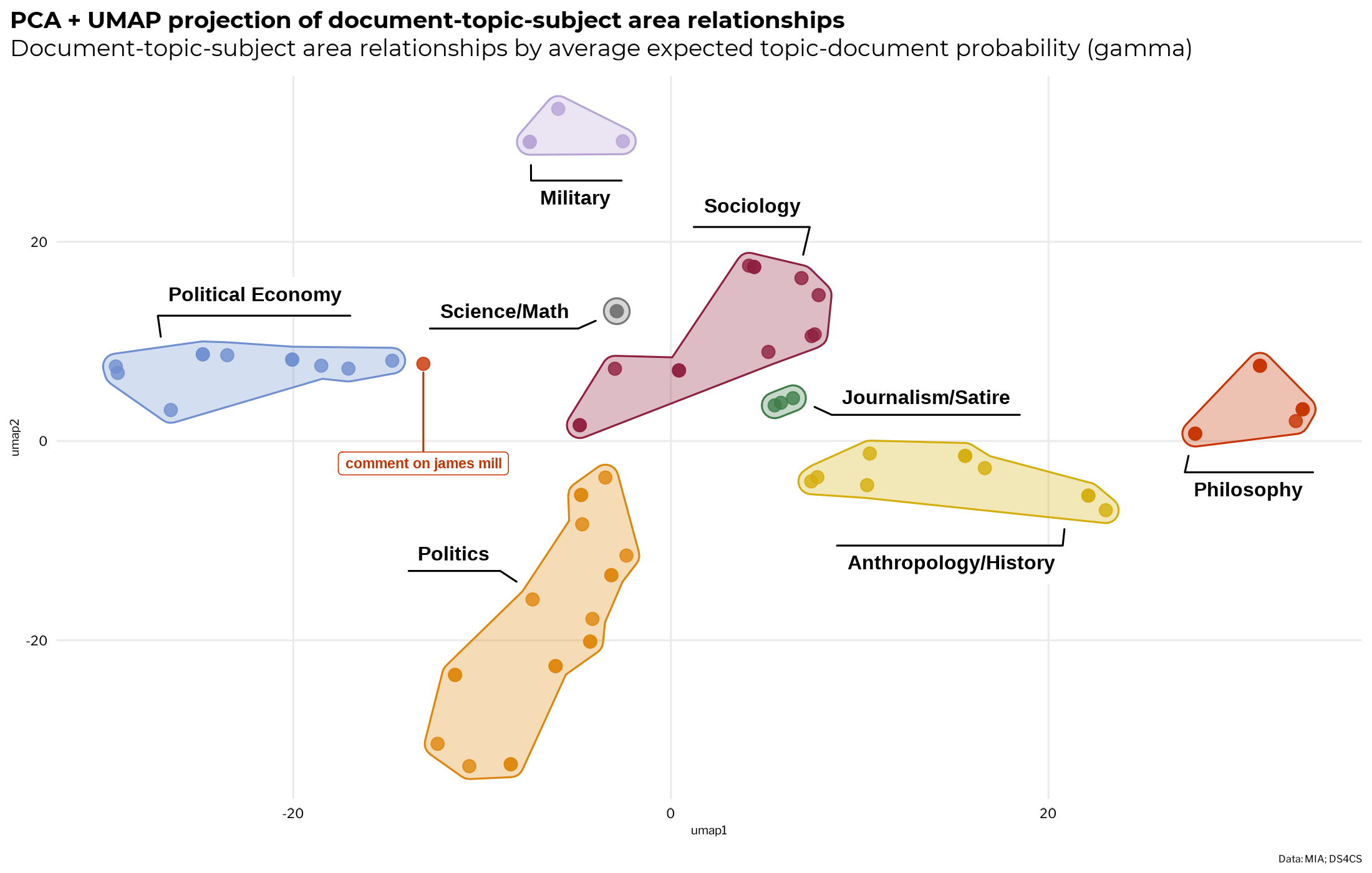
Since the only anomaly is one short text with a minor place in the corpus, the document to category mappings look good. If this chart displays lots of oddly interspersed document clusters, even after UMAP has been tuned to give a good view of the data, it could be (this depends on your data) an indication of problems with the model or topic labeling process.
Visualizing term-topic-label (beta) relationships
Following a nearly identical procedure as the one above, this time with the beta matrix, we can also get a higher-order view of how the actual words or tokens in the model are associated to topics via their category labels. Since each topic is actually a distribution over all words in the model, tidying the beta matrix returns a very long table with n * dictionary size rows, most of which will be near zero.
To get only the terms that are the most related to their parent categories, the average topic-term probability (beta) is calculated according to each topic’s category label. The top 1200 terms in the model by average beta are taken because re-running UMAP over and over as you tune it can take a very long time with larger data sets.
The visualization of the UMAP projection of term-topic-category relationships shows how the terms are used by the authors in relation to different subject areas. One can see how the terms tend to group into broad thematic clusters that are mixed by subject area but dominated by terms from one category.
The anthropology/history cluster is bisected in the middle by small sub-cluster of terms from sociology, philosophy, and natural science. Political economy and sociology are are partially submerged in each other, almost as if a topical venn diagram. Discussion of politics is heavily interspersed with words from topics related to journalism, sociology, and military affairs.
While terms from topic related to journalism are found in the other clusters, the journalism-dominated terms tend to cluster on their own, which makes sense, since these works are often referring very specificly to contemporary people and events that are not likely to appear much in other topics.
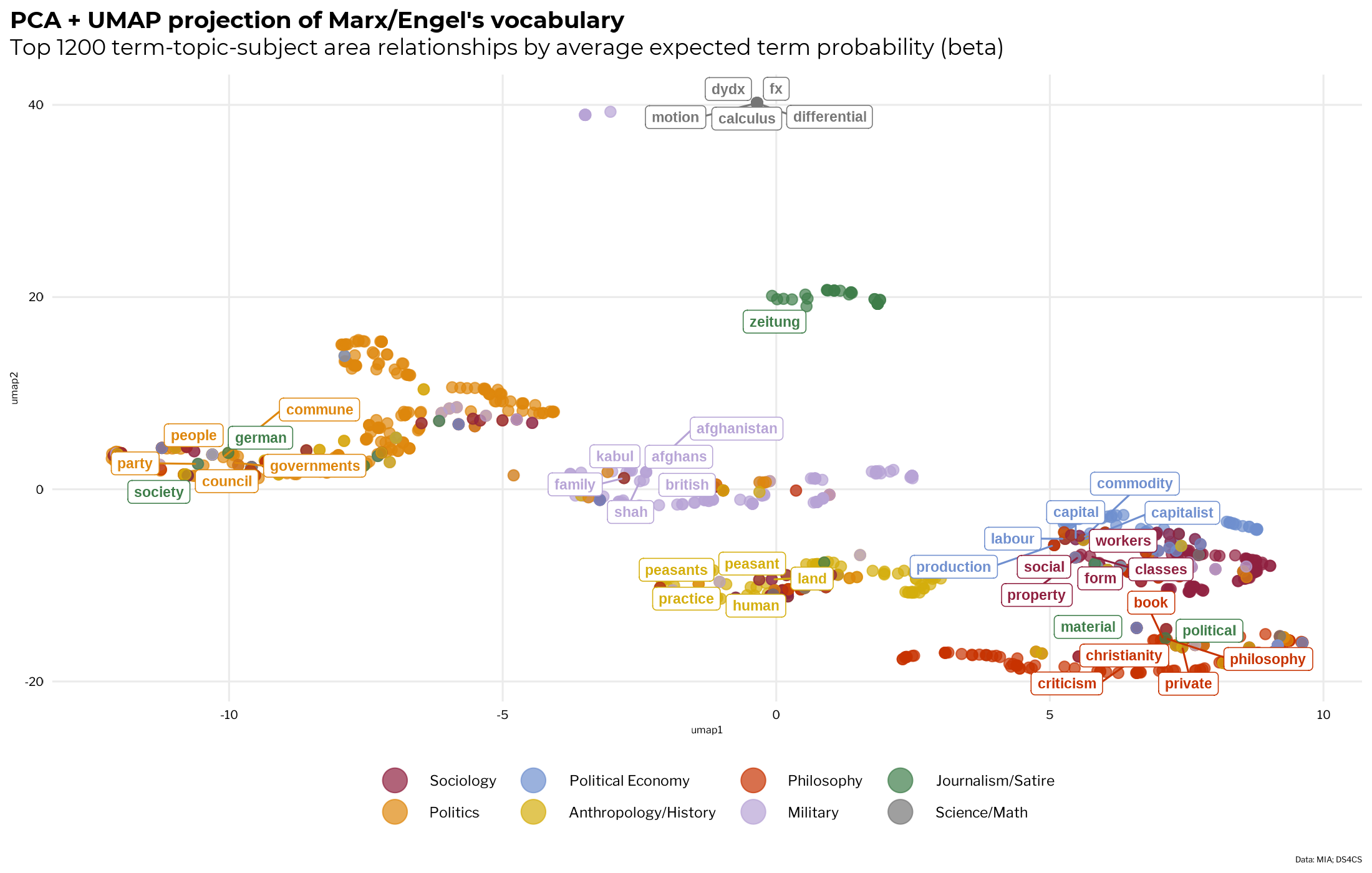
If either (1) the terms do not tend to form groups at all or (2) tend to cluster together in seemingly random and/or unintuitive ways, it could be (depending on the original data) an indication that there is something fishy going on with the model or the process of labeling the topics.
Taking a closer look at the topic labels in the Marx-Engels model
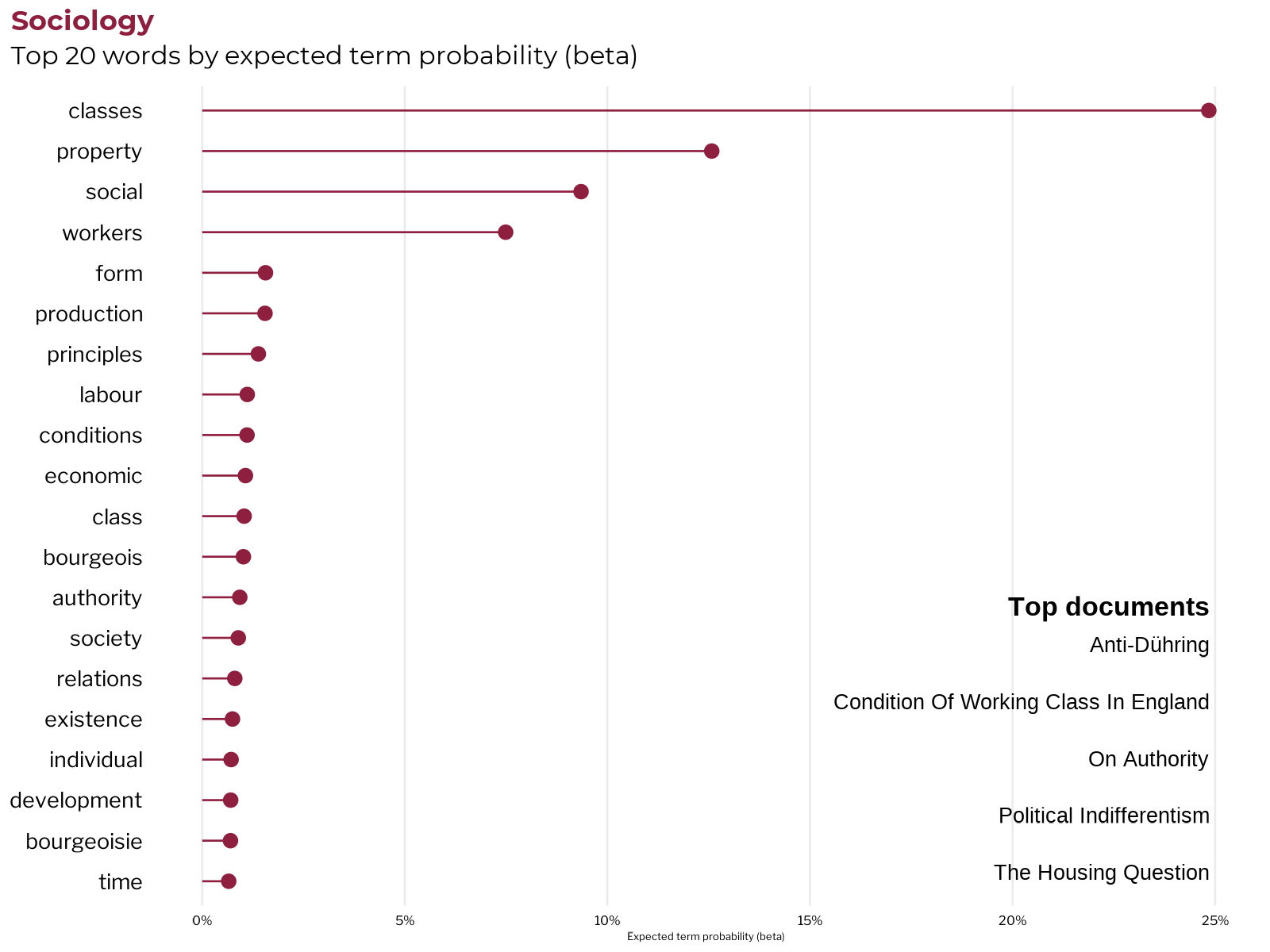
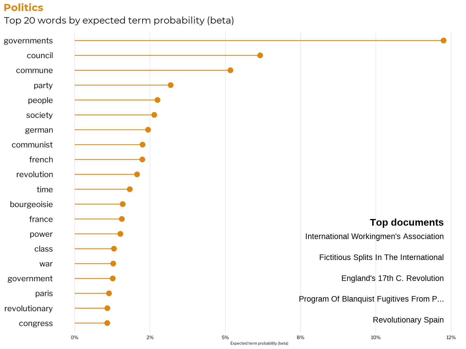
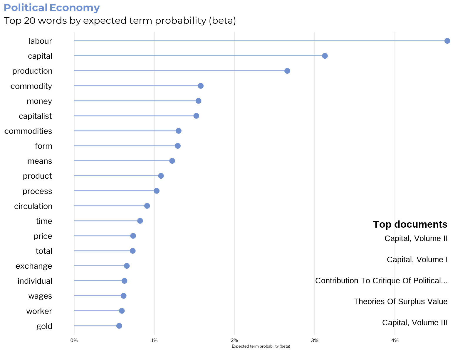
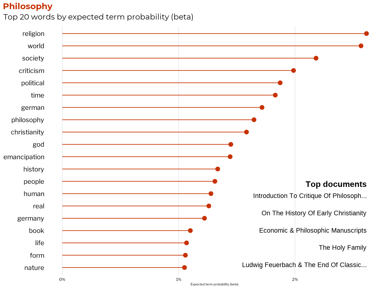
Now that we have had a bird’s eye view of the ways that the terms, topics, and documents relate to the topic labels, it’s time to take a more detailed look at the most important terms and documents to a few of our major category labels. The charts below display the top 20 terms by the average term beta and the top 5 documents by average gamma for each subject area category. Taking a look at the top terms and documents will allow us to judge if the assigned topic labels have grouped the topics together in a conceptually meaningful manner.
# Take the top 5 documents by average gamma
top_docs <- me_tidy_gamma %>%
  group_by(document, category) %>%
  summarise(gamma = mean(gamma)) %>%
  group_by(category) %>%
  slice_max(gamma, n = 5, with_ties = FALSE) %>%
  group_by(category) %>%
  summarise(
    document = str_to_title(document),
    document = str_replace_all(document, "Ii", "II"),
    document = str_replace_all(document, "IIi", "III"),
    document = str_trunc(document, width = 40),
    top_docs = paste(document, collapse = "\n")) %>%
  select(category, top_docs)

# Take the top 20 terms by average beta
beta_cats_tidy <- me_tidy_beta %>%
  mutate(topic = as_factor(topic)) %>%
  group_by(category, term) %>%
  summarise(beta = mean(beta)) %>%
  slice_max(beta, n = 20, with_ties = FALSE) %>%
  arrange(-beta, .by_group = TRUE) %>%
  ungroup() %>%
  left_join(cat_colors) %>%
  left_join(top_docs) %>%
  distinct(category, term, .keep_all = TRUE)

beta_cats_tidy
## # A tibble: 160 x 5
##    category             term          beta color   top_docs
##    <chr>                <chr>        <dbl> <chr>   <chr>
##  1 Anthropology/History practice    0.0587 #d4ae0b "Theses On Feuerbach\nOrigin~
##  2 Anthropology/History peasants    0.0303 #d4ae0b "Theses On Feuerbach\nOrigin~
##  3 Anthropology/History peasant     0.0202 #d4ae0b "Theses On Feuerbach\nOrigin~
##  4 Anthropology/History time        0.0197 #d4ae0b "Theses On Feuerbach\nOrigin~
##  5 Anthropology/History production  0.0190 #d4ae0b "Theses On Feuerbach\nOrigin~
##  6 Anthropology/History human       0.0183 #d4ae0b "Theses On Feuerbach\nOrigin~
##  7 Anthropology/History labour      0.0180 #d4ae0b "Theses On Feuerbach\nOrigin~
##  8 Anthropology/History hand        0.0180 #d4ae0b "Theses On Feuerbach\nOrigin~
##  9 Anthropology/History development 0.0174 #d4ae0b "Theses On Feuerbach\nOrigin~
## 10 Anthropology/History land        0.0174 #d4ae0b "Theses On Feuerbach\nOrigin~
## # ... with 150 more rows
Sociology
Though he did not explicitly frame his work as such, Karl Marx is widely considered to be one of the major figures of classical sociology. The terms most associated with the sociology category cover many of the key concepts in Marx’s approach to sociology, including conflict-theory that demonstrates that society based on private property is necessarily composed of contending social classes. The sociological essence of Marx’s critique of capitalist society is that capitalist social relations of production are founded on the contradictory class interests of workers and the bourgeoisie, who monopolize ownership of society’s means of production.
It’s interesting to note that while Marx wrote vastly more about sociology than Engels by volume, the most associated works are all written by Engels. This makes sense, as Marx was more show and less tell with his methodology, while especially later on in life and after the death of Marx, Engels was taking pains to lay out the scientific socialist method more explicitly as part of their intellectual legacy.
Judgement: Coherent and useful category ✔️
Politics
It’s often under-appreciated how much Marx and Engels wrote about and actually participated in politics. Marx and Engels devoted much of their time, energy, and words to real political movements and engaged in extensive discourse (or more often heated denunciation) with their political contemporaries, allies and rivals alike. As German emigres and former residents of Paris, France, both were especially engaged with the French and German socialist movements.
One strand of their writing about politics deals with their analysis of state power and political theory of revolution. They concluded that governments of capitalist nations were effectively “organizing committees of the bourgeoisie.”
Marx and Engels were particularly influenced by the recent French history of class war and revolution. The experience of the Paris Commune, an embryonic form of proletarian state based on worker’s councils and communes that emerged after a civil war in France.
They theorized that politics was but another battleground in the class war between the working class and the the bourgeoisie. As such, they argued for and actually participated in organizing a communist party to assert the power of the proletariat by fomenting revolution.
Judgement: Coherent and useful category ✔️
Political Economy
The area that one-sided interpretations of Marx as economic determinist tend to overemphasize, by average model expected topic probability, is third place to sociology and politics.
The top terms in this subject touch on many of the key concepts in Marx’s critique of capitalist political economy, including the exploitation of labour by capital, the commodity form, the money form and the money commodity gold, exchange value, the role of exchange and circulation in the system, the formation of prices and wages, working time. socially necessary labour time.
Although topics related to political economy and sociology share many terms and co-habitate in many of the same documents, the strongest document associations for this category all point to Marx’s major works on the topic, including the three parts of Capital along with Theories of Surplus Value.
Judgement: Coherent and useful category ✔️
Philosophy
Marx was originally trained as a philosopher, writing a doctoral dissertation on materialism versus idealism in Greek philosophy. One of Marx’s main accomplishments in the discipline is the development of a philosophical approach that is materialist (as opposed to idealist), historical (as opposed to ahistorical), and dialectical (as opposed to one-sided and mechanical).
Marx and Engels' historical materialist method for the study of human society was based on the analysis of the real history of that form of society. As a materialist philosophy, the Marxist method considers how human society exists in a dialectical relationship with nature.
Their approach to philosophy sought not just to understand, but also to change the world by demonstrating the necessity of revolution. As such, it is a human centered philosophy, whereby people (specifically, the working class and it’s allies) have the agency to change the course of history, but not under conditions of their own choosing. It is a universalist approach in that the emancipation of the working classes marks the emancipation of all people from class society itself.
Marx and Engels also wrote a number of works criticizing the role of religion in perpetuating the oppression and exploitation of class-based societies, whereby the ruling classes of those societies invoke god to ideologically justify their class rule. Many of these works on religion come out of their early engagement and debates with the Young Hegelians, a school of German liberal philosophy that a young Marx belonged to before leaving Germany.
It’s notable that the verb criticism lands in the 5th most associated term: criticism or critique in the classical philosophical sense is one of the most important methodological tools that Marx and Engels use to derive their scientific critique of capitalism.
Judgement: Coherent and useful category ✔️
Working with STM metadata as covariates
Estimating regression effects for model covariates
As mentioned earlier, one of the biggest improvements of structural over conventional topic modeling is the option to include other variables in the model as covariates. Using the estimateEffect function, regression parameters are estimated for each topic-covariate relationship. The option to statistically test the model output against variables representing real world data is extremely helpful for validating the usefulness of the topic model.
The user specifies specify the topics and covariate effects to estimate with the formula argument. Non-linear relationships can be indicated by calling a spline function on numeric covariates with s(). The model parameters can be tidied using the tidy method added by tidytext.
set.seed(1917)
stm_prep <- estimateEffect(1:50 ~ author + s(year),
                           stmobj = me_stm.fit,
                           metadata = me_stm.fit$meta,
                           uncertainty = "Global")
It looks like there are only a few significant effects estimated based the ME model. Think about how the estimates relate to what you already know about the original texts. This finding suggests that overall, there wasn’t much variance between the topics chosen by Marx, those chosen by Engels, and those used when they were both writing. Additionally, for most topics, there didn’t appear to be much variance over time, meaning that they drew across a balanced mix of the majority of topics over the years. Given the topical diversity revealed in the ME canon by the model and domain knowledge of the original texts, this finding seems to be quite reasonable.
stm_prep_tidy <- tidy(stm_prep)
stm_prep_tidy %>% filter(p.value <= .05)
## # A tibble: 7 x 6
##   topic term                      estimate std.error statistic p.value
##   <int> <chr>                        <dbl>     <dbl>     <dbl>   <dbl>
## 1    24 s(year)9                     0.965    0.471       2.05 0.0451
## 2    24 s(year)10                    0.413    0.179       2.31 0.0246
## 3    30 s(year)2                    -0.426    0.198      -2.15 0.0357
## 4    32 s(year)1                     0.510    0.233       2.19 0.0324
## 5    45 authorK. Marx & F. Engels    0.131    0.0461      2.85 0.00609
## 6    46 s(year)8                     0.509    0.228       2.23 0.0298
## 7    49 s(year)8                     0.480    0.224       2.15 0.0361
The model finds a significant positive relationship between the publication year and topic 24 on peasants and pre-capitalist societies, meaning that ME were more likely to write about this topic as time goes on. This appears to track with scholarship on Marx’s late-life intellectual activities.
The model also indicates that ME were more likely to write about topic 45 when writing together, which checks out, since the topic refers to aspects of the critique of political economy (exchange, circulation, turnover) that are dealt with at length in the latter two editions of Capital, which were compiled from Marx’s notes and outlines by Engels after the death of Marx.
Using tidystm for enhanced model effect visualization
The stm package does add methods to plot() to visualize the regression effects. However, it’s possible to escape the limitations of base R plotting by using the tidystm package to extract the effects in tidy format which can easily be plotting with ggplot2.
library(tidystm)
sig_effects_tidy <- extract.estimateEffect(x = stm_prep,
                                           covariate = "year",
                                           model = me_stm.fit,
                                           method = "pointestimate",
                                           labeltype = "prob",
                                           n = 3)
According to the function documentation, all other covariates other than the one indicated by the string provided to covariate are held at their median. So to make a plot of the author effects, one would have to call extract.estimateEffect() again with covariate = "author".
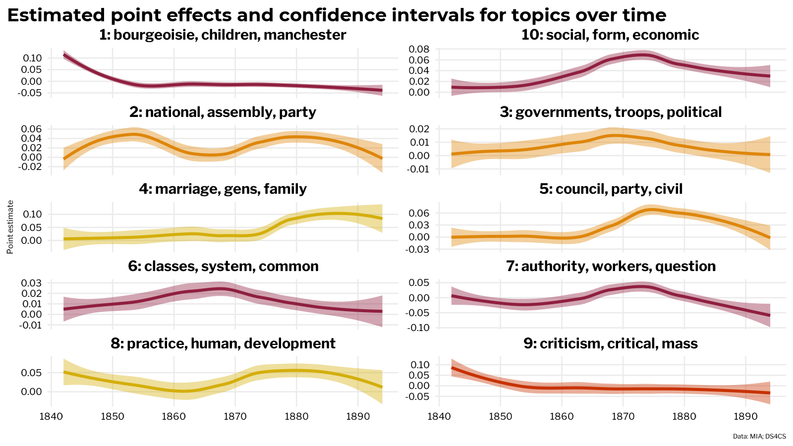
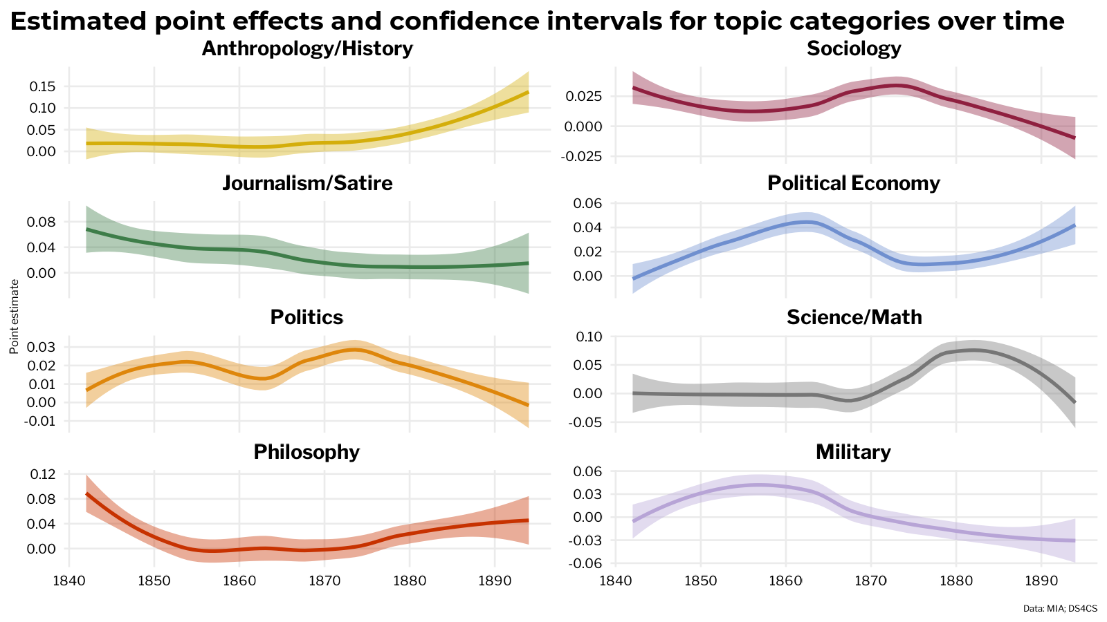
By joining the tidied model effects with the categories labels applied to the topics, it’s also possible to plot the topic effects over time when aggregated by topic category.
Tidy model output with metadata covariates
Topic modeling with stm offers an additional avenue for working with model covariates: the tidy gamma matrix. Covariates are incorporated into the model via their association with the documents in the model. Grabbing the tidy gamma matrix, representing the document-topic probabilities, with tidytext automatically includes the model metadata variables.
gamma_auth <- stm_gamma %>%
group_by(author, topic) %>%
summarise(gamma = mean(gamma)) %>%
mutate(topic = factor(topic)) %>%
# left_join(me_beta_topterms) %>%
left_join(topic_labels) %>%
slice_max(gamma, n = 15) %>%
ungroup() %>%
mutate(topic = reorder_within(topic, gamma, author))
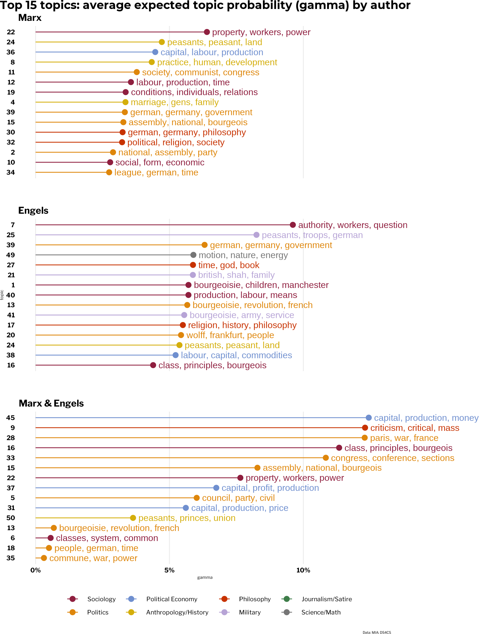
gamma_auth
## # A tibble: 45 x 5
##    author topic      gamma category             color
##    <fct>  <fct>      <dbl> <chr>                <chr>
##  1 Marx   22___Marx 0.0640 Sociology            #8f1f3f
##  2 Marx   24___Marx 0.0471 Anthropology/History #d4ae0b
##  3 Marx   36___Marx 0.0447 Political Economy    #6F8FCF
##  4 Marx   8___Marx  0.0434 Anthropology/History #d4ae0b
##  5 Marx   11___Marx 0.0378 Politics             #de860b
##  6 Marx   12___Marx 0.0356 Sociology            #8f1f3f
##  7 Marx   19___Marx 0.0336 Sociology            #8f1f3f
##  8 Marx   4___Marx  0.0336 Anthropology/History #d4ae0b
##  9 Marx   39___Marx 0.0333 Politics             #de860b
## 10 Marx   15___Marx 0.0328 Politics             #de860b
## # ... with 35 more rows
To associate metadata with terms related to topics, the tidy gamma matrix can be joined to the tidy beta matrix by topic. Once they’re together, it’s easy to create visualizations that go far beyond what base R plotting with stm methods are capable of creating. Below, the top topics for each author are plotted by average document-topic probability (gamma) and colored by the topic discipline category. It appears to lend more credence to the regression finding