Tidy Text Scraping, Cleaning and Processing with Karl Marx and R
This is the introductory unit in a practical learning series on using text-as-data for socialist purposes. In this tutorial, I will introduce readers to three tidy methods of scraping, cleaning, and processing text from common sources and in the process build a tidy corpus of machine readable Marxist texts based the three volumes of Karl Marx’s Capital. The lesson will cover how to scrape text data from three of the most common sources: html webpages, pdf documents, and MS Word documents. All three books, and the rest of the texts used in this course, are public domain and hosted by the Marxists Internet Archive.
Whenever possible, I try to follow tidy data principles and operate within the tidyverse ecosystem of packages when working in R. The essential structure of tidy data are variables in columns, observations of those variables in the rows, and one data point per observation per each row.
In this tutorial, I’ll show a tidy approach for working with text that includes scraping, cleaning, processing, and visualization. I am hardly an expert programmer, so this is meant to be a practical exercise for budding citizen socialist data scientists in gathering and preparing data. The vibe we are going for is “if I can do it, so can anyone!”
Actual experts Julia Silge and David Robinson have written an excellent free e-book covering many aspects of tidy approach to text mining using R. So if you are really interested in text mining for your own interests or purposes, I highly recommend reading that book first. If you want to get a head start on the more advanced stuff, check out this also free book on supervised machine learning for text analysis by Emil Hvitfeldt and Julie Silge. But first, you actually need some text to analyze! So let’s press onward.
Table of Contents
Scraping text three ways from the Marxists Internet Archive
Often, it’s quite simple to download some data contained in a .csv or .xlsx, import it into some data analysis software, and get started. Unfortunately, the majority of text data isn’t gift wrapped in such a manner, though there are ways to get pre-prepared text, for example, public domain books with the gutenbergr package
An unimaginable amount of text data exists in the world and very much of it is available online in both obvious and obscure forms. This tutorial demonstrates how to scrape text data from three of the most common containers for text in the digital age:
- html webpages
- PDF documents
- MS Word documents.
Since the aim of this tutorial is to build a corpus (a fancy way of saying a body of text) of Marxist texts, we’ll be scraping the three volumes of Marx’s Capital from the Marxists Internet Archive, the internet’s biggest open access repository of Marxist works. The MIA offers text stored in many different formats, including html, .pdf, and .doc files, including several other e-book formats that we won’t touch on for now.
In the lesson that follows, we’ll learn how to use a tidy workflow to scrape, clean, and process the three volumes of Capital: Volume I from html text, Volume II from a pdf file, and Volume III from a Word document. To finish, we’ll explore the tidy corpus of Marxist texts for a quick demonstration of how tidy text can be counted, summarized, used to compute summary statistics, and included in simple models.
The importance of ethics when scraping the web for data
Reminder that scraping data can have real world ethical implications and, in some jurisdictions like Canada, legal consequences. It’s beyond the scope of the article to go into this in too much detail. Suffice it to say, before you scrape, it’s worth asking yourself some questions about the ethics and legality of data scraping in the given context and doing a bit of investigation if needed.
Many websites will have a robot.txt file that will define what actions simulated users or bots can undertake. It’s possible to break a website by accidentally by simulating a denial-of-service (DOS) attack with an overwhelming number of requests at very high speeds; a user can only click so many links in a given time, while a machine can do it exponentially faster. Typically, robots.txt will define a delay time between crawl actions in order to limit requests to a reasonable volume and prevent their servers from being overwhelmed.
In the case of the MIA, it seems quite reasonable to assume that scraping is perfectly allowable. The site admins address scraping in the site FAQ and suggest several methods for doing so. The admin of MIA stipulate a crawl delay in their FAQ: “Note that you must limit your download to reasonable rates (request interval ca. 500ms — 1 second).”
Capital Volume I: Tidy and responsible web scraping with rvest and polite
The fundamentals of importing html text into R
First at the plate for scraping is text data stored on html webpages. Imagine how much text data in html form exists in the world: basically every website that exists as at least some text in it and many of the have lots of text. Learning how to scrape data of all kinds from the web is an essential skill for any citizen data scientist.
Below, I’ll show a basic tidy workflow for scraping and cleaning text from html files with the rvest package, which is part of the tidyverse community of packages. By the end of this section, you will have a good impression of the main benefits of using a tidy approach to web scraping with tidyverse verb functions like mutate or filter from dplyr as well the pipe operator %>% from magrittr.
Begin by loading the required packages for the scraping and cleaning process. If you find that the code in this unit doesn’t work for you, it’s likely due to differences in versions of packages. You can download an .rds R data file here that contains a dataframe with the specific package versions used to create this document.
pacman::p_load(tidyverse, tidytext, glue, here, update = FALSE)
A tidy scraping workflow begins with a file path or more likely a URL to retrieve the html from. There is a basic workflow that applies in general situations, which is something like: (1) retrieve html object; (2) select relevant html nodes and elements; (3) parse the required text from the html; (4) clean and tidy the text. Of course, the particulars of the process will depend greatly on the website and your purpose for scraping it to stat with. Since websites are extremely numerous and are built in so many different ways, one will encounter many, many different structures of html when attempting to scrape.
For this reason, some sites will be rather simple to scrape, while pulling the data from others can be a real hassle. One of the big benefits of tidy scraping is the versatility and power of tidyverse style packages for manipulating data. Tidy scraping allows for flexible use of those tools to adapt to the many unexpected twists and turns of poorly structured or written html webpages that one inevitably finds out there.
Fortunately, the Marxists Internet Archive is pretty amenable to scraping with consistently structured index pages for authors and works that facilitate easy scraping. There are differences in how the text is stored across author pages, which could be a problem for scraping multiple authors at a time, but that’s a problem for another time.
On the MIA, each author and most author’s major, multi-chapter works have a page that indexes links, ending in "index.htm", either to the raw texts themselves or to other index pages. To scrape a book from the MIA, start by copy and pasting the URL to the book’s index page, as done below. Importing the page’s html file into R is as simple as calling rvest::read_html() on the page URL.
# Get the URL
c1_index_url <- "https://www.marxists.org/archive/marx/works/1867-c1/index.htm"

# Get index html
c1_index_html <- read_html(c1_index_url)
c1_index_html
## {html_document}
## <html>
## [1] <head>\n<meta name="viewport" content="width=device-width, initial-scale= ...
## [2] <body> \r\n<p class="title">Karl Marx</p>\r\n<h1>Capital<br><span style=" ...
A note on the impernanence of existence and also XML objects in R
The output of read_html() is a special class of object meant to represent html documents in R using the form of XML or extensible markup language, which is specifically designed for sharing a wide variety of structured data types. The html document output produced by rvest is a list of html documents that contains the head and body html nodes of the web page.
Under the hood, rvest is built on top of the xml2 package and that html document is really an xml_document class object, which is a list of composed of an XML document and XML nodes. You don’t need to know much about XML documents to be able to work with them to scrape data from them, but there is one essential quirk of the object class to mention up front.
An xml_document use external pointers to represent the data, which means they are not permanent and can only be used in the same R session they are created within. That means that these objects cannot be saved as .rds files and then imported again for future use. Not being able to use the objects from one session to another creates a barrier to producing reusable and reproducible code. More on how to solve this problem will follow shortly.
c1_index_html %>% class()
## [1] "xml_document" "xml_node"
Finding the desired data by targeting html with a web browser
It isn’t necessary to have a deep understanding of how html and css (cascading style sheets) work in order to succeed at web scraping. Generally, one only needs to know enough to be able to locate the data you want to target and know how to tell the rvest functions to select and extract it. A good review of the basic knowledge needed to start scraping can be read here.
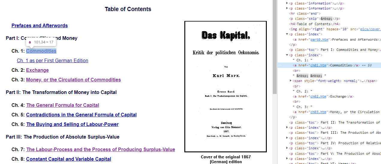
The best way to get started is by inspecting the html and css structure of the webpage that you want to scrape. One of the easiest ways to do this is to use inspect mode (F12 by default on most browsers) in your web browser of choice. Inspect mode give provides all sorts of information on what’s going on behind the scenes on a given webpage, including the html code used to build it. Using the pane of the right, search through the html structure of the site and locate the elements with the data targeted for scraping.
In the case of the Capital Volume I index site, we can see that the links and chapter titles are contained within paragraph nodes (tagged with <p>) with the class "index", in child elements that are tagged with <a>, denoting a hyperlink. The chapter link is contained within the sub-node attribute "href", while the chapter title text is contained within the node itself.
Some people swear by using selectorgadget, a Chrome browser extension that will allow the user to generate CSS selectors to input into rvest’s html_ family of functions to select html nodes and attributes. Often it will at the very least produce a good starting point for finding the specific selector or path that you need.
Scraping an entire book using dynamic link generation
Quite often, when scraping data from the web, it will be necessary to gather it from more than just one website at a time. There are a few methods for doing this using a tidy workflow, but we’re going to cover the most direct one, scraping multiple pages by iterating read_html() over a series of links. Now that we know where the chapter links are stored in the Capital Vol. I index page, it’s possible to extract them and produce a data frame of links to feed into read_html().
Commence by using rvest’s html_nodes() function to select the page nodes that are tagged as hyperlinks with "a", then pipe %>% the output into html_attr to access the chapter links within the node element "href". In this case, we end up with the tail end of each link relative to the base URL of the book index page. The MIA also links to other content on book index pages such as other file formats for the text, external or biographical sources, audio, pictures, video, and so on.
library(rvest)
# Convert index html into tibble of text links
c1_links <- c1_index_html %>%
  html_nodes("a") %>%
  html_attr("href") %>%
  as_tibble() %>%
  rename(chapter = value)

c1_links
## # A tibble: 55 x 1
##    chapter
##    <chr>
##  1 ../download/pdf/Capital-Volume-I.pdf
##  2 ../download/doc/Capital-Volume-I.doc
##  3 ../download/zip/Capital-Volume-I.zip
##  4 ../download/epub/capital-v1.epub
##  5 ../download/mobi/capital-v1.mobi
##  6 ../download/prc/capital-v1.prc
##  7 part0.htm
##  8 ch01.htm
##  9 commodity.htm
## 10 ch02.htm
## # ... with 45 more rows
The MIA has a consistent format for linking to chapter pages of major works, which is something like: book index url / chapter number.htm. It is therefore possible to easily filter out all of the non-chapter text links simply by using filter() and str_detect() to filter chapter for only rows with strings that begin with "ch". The result is a dataframe column that contains just the last part of the link prior to the final “/” in the URL. We can use glue() to paste the tail of the link into the base URL of the book index to produce a working link relative to the base URL of the site.
c1_links <- c1_links %>%
  filter(str_detect(chapter, "^ch.+")) %>%
  mutate(link = glue("archive/marx/works/1867-c1/{chapter}"))

c1_links
## # A tibble: 33 x 2
##    chapter  link
##    <chr>    <glue>
##  1 ch01.htm archive/marx/works/1867-c1/ch01.htm
##  2 ch02.htm archive/marx/works/1867-c1/ch02.htm
##  3 ch03.htm archive/marx/works/1867-c1/ch03.htm
##  4 ch04.htm archive/marx/works/1867-c1/ch04.htm
##  5 ch05.htm archive/marx/works/1867-c1/ch05.htm
##  6 ch06.htm archive/marx/works/1867-c1/ch06.htm
##  7 ch07.htm archive/marx/works/1867-c1/ch07.htm
##  8 ch08.htm archive/marx/works/1867-c1/ch08.htm
##  9 ch09.htm archive/marx/works/1867-c1/ch09.htm
## 10 ch10.htm archive/marx/works/1867-c1/ch10.htm
## # ... with 23 more rows
Now we have a tibble of links that can be used to scrape the html of all the chapter pages in sequence. In this case, the links had a short and consistent format and they could have been cobbled together with something like paste0("ch", 1:n_chapters, ".htm"). However, very often you will need to iteratively scrape links to pages with URLs that do not share the same neat, consistent format. In those rather common situations, the method of dynamically scraping the links from their index page shown above will work just as well to generate more complex links.
On the necessity of using map() with rvest for vectorized dataframe operations
As we saw above, scraping html from one URL at a time is quick and simple. Simply place the URL into the read_html function and then retrieve the html on the other end. If you need to scrape one page or maybe a handful or pages as a one-time deal, no problem.
# Test with the first two links
test_links <- c1_links %>%
  slice(1:2) %>%
  mutate(full_link = glue("https://marxists.org/{link}"))

# Testing a single link
test_links$full_link[[1]] %>% read_html()
## {html_document}
## <html>
## [1] <head>\n<meta name="viewport" content="width=device-width, initial-scale= ...
## [2] <body>\r\n<p class="title">Karl Marx. Capital Volume One\r\n<a name="000" ...
However, trying to do the same operation using a vector of multiple links, like a dataframe column, to scrape a html object for each link will not work. It throws an error because read_html(), despite being part of a core tidyverse package, will not work with vectorized dataframe operations. This is probably because the xml_document output is necessarily a list, which can’t be placed into a dataframe column by mutate when called like so.
test_links %>%
  mutate(html = read_html(full_link))
## Error: Problem with `mutate()` column `html`.
## i `html = read_html(full_link)`.
## x `x` must be a string of length 1
As the error tells us, read_html() only works on a single URL or connection at a time. In order to iterate over a series of links in a tidy workflow and place a list within a dataframe column, it’s necessary to nest the call to read_html() within map, providing the unquoted name of the dataframe column as the .x argument to map(). Doing this will add a list column to the dataframe that contains the html source for each link.
test_links %>%
  mutate(html = map(.x = full_link, .f = read_html))
## # A tibble: 2 x 4
##   chapter  link                                full_link                  html
##   <chr>    <glue>                              <glue>                     <list>
## 1 ch01.htm archive/marx/works/1867-c1/ch01.htm https://marxists.org/arch~ <xml_~
## 2 ch02.htm archive/marx/works/1867-c1/ch02.htm https://marxists.org/arch~ <xml_~
Responsibly scraping many web pages with polite and nod()
As mentioned earlier, it’s possible to do real harm by overwhelming a server with a flurry of requests, the dreaded infinite request loop being the worst of all. Manually scraping one URL at a time will pretty much never overtax a server. However, when one starts using software to automatically scrape multiple pages iteratively to extract large amounts of data, it’s important to be as responsible as possible.
Using the polite package makes the process of web scraping in an ethical way much easier. Using the bow() function will establish a user agent session with the MIA server and automatically read the site’s robots.txt file (if one exists) to establish permissions for the setting; the output is a special polite class of R object designed to represent a polite user agent session with a given server. Once the session is established, you just have to call the scrape function on the session object to scrape the html.
library(polite)
test_session <- bow("https://www.marxists.org/archive/marx/works/1867-c1/archive/marx/works/1867-c1/ch01.htm")
test_html <- scrape(test_session)
test_html
## {html_document}
## <html>
## [1] <head>\n<meta name="viewport" content="width=device-width, initial-scale= ...
## [2] <body> \r\n<blockquote>\r\n<p class="title">\r\nMarxists Internet Archive ...
Below, we define a function to combine the mutate, map, read_html method of creating a dataframe list-column of html objects with the polite scraping functions of bow, nod, and scrape. Establishing a session and setting a delay like so means that you won’t ever accidentally slam a server with requests.
- The only input to the function is a dataframe containing links from a MIA index page
index_df. - A base user session is established with the MIA server using
bow(). As per the request of the MIA site admins, a one second crawl delay is set with thedelay = 1argument. - If no delay is provided,
politewill default what is in robots.txt, or if not present, a reasonable default rate. - To set a crawl rate, you need to identify yourself to the server by providing a user agent string to the
user_agentargument. - The
nod()function is used to modify the base session to access other parts of the site. The first argument is thepolitesession object and the second is a path or URL that is relative to the base session URL. - The output of
nod()is a modifiedpolitesession object, which is piped directly intoscrape()to extract the html. - To scrape this text, you need to specify a charset encoding within
scrape()other than the default of UTF-8. This is done by providing the content format and encoding to thecontentargument. If you run into encoding problems scraping html,guess_encoding()fromrvestmay be able to help pick one. - The scraping process is wrapped in
try(x, silent = TRUE)so that the process of scraping many links isn’t interrupted by an error if one of the links can’t be scraped. By default,try()will return the output of errors asNA.
polite_scrape <- function(index_df) {
  require(polite)

  #  Create a base user agent session with MIA
  mia_session <- bow("https://www.marxists.org/",
                     user_agent = "DS4CS <https://ds4cs.netlify.app>",
                     delay = 1)

  # Use nod to iterate over each link in index_df and scrape
  index_df %>%
    mutate(html = map(.x = index_df$link,
                      .f =
                        ~ try(nod(bow = mia_session,
                                  path = .x) %>%
                                scrape(verbose = TRUE,
                                       content = "text/html; charset=ISO-8859-9"),
                              silent = TRUE)
                      )
           )

}
To establish a session and scrape the html for each link into a list-column, just call polite_scrape() on the dataframe of links. Since this is scraping 33 chapters worth of html, it might take a few minutes to finish scraping.
c1_html <- c1_links %>%
  polite_scrape()
Inspecting the data frame, we have a list-column of xml objects; essentially a list of lists, which makes it a bit trickier to work with than a conventional dataframe column.
c1_html$html %>% head(3)
## [[1]]
## {html_document}
## <html>
## [1] <head>\n<meta name="viewport" content="width=device-width, initial-scale= ...
## [2] <body>\r\n<p class="title">Karl Marx. Capital Volume One\r\n<a name="000" ...
##
## [[2]]
## {html_document}
## <html>
## [1] <head>\n<meta name="viewport" content="width=device-width, initial-scale= ...
## [2] <body> \r\n\r\n<p class="title">Karl Marx. Capital Volume One</p>\r\n\r\n ...
##
## [[3]]
## {html_document}
## <html>
## [1] <head>\n<meta name="viewport" content="width=device-width, initial-scale= ...
## [2] <body> \r\n\r\n<p class="title">Karl Marx. Capital Volume One</p>\r\n\r\n ...
How to save html objects in R for reusable scraping code
Recall the earlier discussion of the impermanence of xml_document objects in R. Since the object is represented by an external pointer (externalptr in R) it can only exist within the span of one R session. That means that if you tried to save these objects as an .rds R data object, they would be non-functional upon import. Running any sort of operation on them will only return an invalid external pointer error. For many reasons, it will be desirable to have access to the html objects without having to download them again. It will be impossible to write reproducible and reusable scraping code, nor proceed with much else that uses the scraped objects. Scraping tons of data from many webpages can sometimes take hours to complete, so it’s absolutely essential to have easy access to it if that data is going to be useful in the future.
The workaround to this is simply to save the xml_document objects containing the scraped html into actual .html files in storage in some external location. Below, we define a function to take a dataframe with a list-column of html objects and writes them to disk. In this case, there is one html document for every chapter scraped, so each chapter is written as a separate .html file. Again, the writing process is wrapped in try(silent = TRUE) to keep an error from stopping the operation. If you are writing a large number of html files, try() is also a necessity, since one file with bad encoding in a batch of 10000 files can jam the process up with an error at any time.
# Write HTML files to disk
ds4cs_writehtml <- function(df) {
  require(xml2)

  html <- df[["html"]]
  filenames <- paste0("capital_vol1_", df[["chapter"]])

  walk2(html, filenames, ~ try(write_html(
    x = .x,
    file = here(
      'ds4cs_working',
      'posts',
      'd5_text_analysis_marxism',
      'data',
      'scraping_lesson',
      paste0(.y)
    )
  ), silent = TRUE))

}

ds4cs_writehtml(c1_html)
The scraped html can now be accessed anytime without having to download it all over again. However, the html still needs to be read into R using read_html() after every time it’s imported. Here the file paths for the saved html are converted into a tibble.
html_paths <-
  list.files(
    here(
      'ds4cs_working',
      'posts',
      'd5_text_analysis_marxism',
      'data',
      'scraping_lesson'
    ),
    pattern = ".htm",
    full.names = TRUE
  ) %>%
  as_tibble() %>%
  rename(html_path = value)

html_paths
## # A tibble: 33 x 1
##    html_path
##    <chr>
##  1 C:/Users/Ryan/Documents/rromard_website/ds4cs_working/posts/d5_text_analysis~
##  2 C:/Users/Ryan/Documents/rromard_website/ds4cs_working/posts/d5_text_analysis~
##  3 C:/Users/Ryan/Documents/rromard_website/ds4cs_working/posts/d5_text_analysis~
##  4 C:/Users/Ryan/Documents/rromard_website/ds4cs_working/posts/d5_text_analysis~
##  5 C:/Users/Ryan/Documents/rromard_website/ds4cs_working/posts/d5_text_analysis~
##  6 C:/Users/Ryan/Documents/rromard_website/ds4cs_working/posts/d5_text_analysis~
##  7 C:/Users/Ryan/Documents/rromard_website/ds4cs_working/posts/d5_text_analysis~
##  8 C:/Users/Ryan/Documents/rromard_website/ds4cs_working/posts/d5_text_analysis~
##  9 C:/Users/Ryan/Documents/rromard_website/ds4cs_working/posts/d5_text_analysis~
## 10 C:/Users/Ryan/Documents/rromard_website/ds4cs_working/posts/d5_text_analysis~
## # ... with 23 more rows
Offline html files can be scraped in the same manner as online webpages. By supplying the file paths in html_paths to read_html() within mutate and map, the html documents are recreated as a list-column in the dataframe of paths. Like before, those objects exist only within the confines of this particular R session, but it’s much easier to access now.
c1_html <- html_paths %>%
  mutate(
    html = map(html_path, ~ read_html(.)),
    chapter = str_extract(html_path, "(?<=ch)\\d+")
  ) %>%
  select(-html_path)
We now have a tidy tibble with one html document per chapter on our hands here. The next step is to actually extract the text out of the html, wrangle it into a useful form, and extract associated metadata like chapter numbers and titles.
c1_html
## # A tibble: 33 x 2
##    html       chapter
##    <list>     <chr>
##  1 <xml_dcmn> 01
##  2 <xml_dcmn> 02
##  3 <xml_dcmn> 03
##  4 <xml_dcmn> 04
##  5 <xml_dcmn> 05
##  6 <xml_dcmn> 06
##  7 <xml_dcmn> 07
##  8 <xml_dcmn> 08
##  9 <xml_dcmn> 09
## 10 <xml_dcmn> 10
## # ... with 23 more rows
This is accomplished with the html_ family of functions from rvest. Inspecting the chapter text page with a web browser in inspect mode, the main text of the book is located in the html body node, within paragraph elements without any tags.
The nodes containing the body text can be accessed with the html_nodes() function, supplying the CSS selector for paragraph elements without class tags as the second argument. This means that we are dropping the book footnotes for now, which are held in elements with the attribute information, since that is often very tricky text to work with. As before when parsing html from a webpage, the function call returns an xml_nodeset object with the html elements containing the text that we want.
test_nodeset <- c1_html$html[[1]] %>%
  html_nodes("body p:not([class])")
test_nodeset
## {xml_nodeset (147)}
## [1] <p> <a name="014"> </a></p>
## [2] <p>\r\nThe wealth of those societies in which the capitalist mode of pro ...
## [3] <p>\r\nA commodity is, in the first place, an object outside us, a thing ...
## [4] <p>\r\nEvery useful thing, as iron, paper, &c., may be looked at fro ...
## [5] <p>\r\nThe utility of a thing makes it a use value.<sup class="enote"><a ...
## [6] <p>\r\nExchange value, at first sight, presents itself as a quantitative ...
## [7] <p>\r\nA given commodity, <em>e.g.</em>, a quarter of wheat is exchanged ...
## [8] <p>\r\nLet us take two commodities, <em>e.g.</em>, corn and iron. The pr ...
## [9] <p>\r\nA simple geometrical illustration will make this clear. In order ...
## [10] <p>\r\nThis common “something” cannot be either a geometrical, a chemica ...
## [11] <p>\r\nAs use values, commodities are, above all, of different qualities ...
## [12] <p>\r\nIf then we leave out of consideration the use value of commoditie ...
## [13] <p>\r\nLet us now consider the residue of each of these products; it con ...
## [14] <p>\r\nWe have seen that when commodities are exchanged, their exchange ...
## [15] <p>\r\nA use value, or useful article, therefore, has value only because ...
## [16] <p>\r\nSome people might think that if the value of a commodity is deter ...
## [17] <p>\r\nWe see then that that which determines the magnitude of the value ...
## [18] <p>\r\nThe value of a commodity would therefore remain constant, if the ...
## [19] <p>\r\nA thing can be a use value, without having value. This is the cas ...
## [20] <p>\r\n <a name="043"> </a> <a name="S2"> </a></p>
## ...
The text can be extracted using either the html_text() or html_text2() functions. The first gives unstructured raw text, while the second does it’s best to represent how the text appears on the page. The majority of the time you will want to use html_text2() to get much cleaner, more orderly text data that can easily be incorporated into a tidy workflow.
test_nodeset %>%
  html_text2() %>%
  as_tibble()
## # A tibble: 147 x 1
##    value
##    <chr>
##  1 " "
##  2 "\r The wealth of those societies in which the capitalist mode of production~
##  3 "\r A commodity is, in the first place, an object outside us, a thing that b~
##  4 "\r Every useful thing, as iron, paper, &c., may be looked at from the two p~
##  5 "\r The utility of a thing makes it a use value.[4] But this utility is not ~
##  6 "\r Exchange value, at first sight, presents itself as a quantitative relati~
##  7 "\r A given commodity, e.g., a quarter of wheat is exchanged for x blacking,~
##  8 "\r Let us take two commodities, e.g., corn and iron. The proportions in whi~
##  9 "\r A simple geometrical illustration will make this clear. In order to calc~
## 10 "\r This common “something” cannot be either a geometrical, a chemical, or a~
## # ... with 137 more rows
Just like read_html(), the rvest functions for extracting the html nodes from the xml_document like html_nodes(), html_elements(), and html_attrs() are also non-vectorized and therefore only work on a single object at a time. This means that in order to work on dataframe columns, calls to these functions should be used within mutate and map as previously demonstrated.
The code below takes us from a dataframe of scraped html objects to a tidy dataframe of text with one row per chapter section in the text. The chapter titles are extracted from the metadata stored in the head node of most html documents, the chapter numbers are also parsed from this information. Finally, the list-columns produced by map() are turned into a longer dataframe with unnest. It’s worth mentioning that html_attrs_dfr() is a very useful way of getting the html attributes out of a node set directly into a dataframe; often this works for extracting difficult to reach text data from the html.
c1_html_text <- c1_html %>%
  mutate(
    text = map(
      .x = html,
      .f = ~ html_nodes(., "body p:not([class])") %>%
        html_text2 %>%
        as_tibble() %>%
        bind_rows()
    ),
    ch_title = map(
      .x = html,
      .f = ~ html_nodes(., "head meta:nth-child(4)") %>%
        html_attrs_dfr() %>%
        select(content) %>%
        unlist()
    ),
    ch_title = str_extract_all(ch_title, "\\(.+\\)"),  # extract text between brackets
    ch_title = str_remove_all(ch_title, "\\(|\\)"),  # remove brackets
    ch_num = parse_number(chapter),
  ) %>%
  unnest(cols = c(text, ch_title)) %>%
  select(ch_num, ch_title, text = value) %>%
  filter(!is.na(text))

c1_html_text
## # A tibble: 1,565 x 3
##    ch_num ch_title    text
##     <dbl> <chr>       <chr>
##  1      1 Commodities " "
##  2      1 Commodities "\r The wealth of those societies in which the capitalist~
##  3      1 Commodities "\r A commodity is, in the first place, an object outside~
##  4      1 Commodities "\r Every useful thing, as iron, paper, &c., may be looke~
##  5      1 Commodities "\r The utility of a thing makes it a use value.[4] But t~
##  6      1 Commodities "\r Exchange value, at first sight, presents itself as a ~
##  7      1 Commodities "\r A given commodity, e.g., a quarter of wheat is exchan~
##  8      1 Commodities "\r Let us take two commodities, e.g., corn and iron. The~
##  9      1 Commodities "\r A simple geometrical illustration will make this clea~
## 10      1 Commodities "\r This common “something” cannot be either a geometrica~
## # ... with 1,555 more rows
Flexible tokenization of tidy text with unnest_tokens()
The Capital Volume I text-data is almost ready for use! Currently, we have a dataframe with a column that contains very long character strings featuring paragraphs and pages worth of text. In order to to make the text both a whole lot easier to clean and also machine readable, those long character strings need to be broken up into smaller pieces referred to as tokens. This process, known as tokenization, is extremely important in the field of text analytics and natural language processing.
Tokens can be any semantically meaningful components of natural language text. To get an idea of the common types of tokens used in language processing, here are the default types of tokens available to the unnest_tokens() function, the workhorse of the tidytext package: characters, character shingles, ngrams, skip_ngrams, sentences, lines, paragraphs, regex, tweets. There are many more options for tokenization beyond those basic methods, but for now, let’s just go with plain old word tokens. By calling unnest_tokens() on our html text tibble, we can turn it into a tidy tibble with one word per row for each word in the document. It’s going to be a long table, but being in tidy form makes it pretty easy to handle.
c1_html_text %>%
  unnest_tokens(word, text)
## # A tibble: 212,897 x 3
##    ch_num ch_title    word
##     <dbl> <chr>       <chr>
##  1      1 Commodities the
##  2      1 Commodities wealth
##  3      1 Commodities of
##  4      1 Commodities those
##  5      1 Commodities societies
##  6      1 Commodities in
##  7      1 Commodities which
##  8      1 Commodities the
##  9      1 Commodities capitalist
## 10      1 Commodities mode
## # ... with 212,887 more rows
A note on tokenization, punctuation, and compound-words
There are some NLP techniques that can actually integrate punctuation and all sorts of non-word symbols. However, for many other language processing purposes (topic modeling for example), it’s standard procedure to remove punctuation from text before or during tokenization. When using unnest_tokens, punctuation is removed automatically unless specified with strip_punct = FALSE.
The common need to remove punctuation can cause some problems, particularly for these texts, because of the abundance of compound words. That is, conjoined words that are separated by a hyphen. So many of Marx’s key words and concepts are described by compound words, two prominent examples being use-value and exchange-value.
Converting the hyphens that are right next to word boundaries (the regular expression "\\b") with underscores is a quick trick for preserving compound words. When punctuation is removed and text is cast into tokens, those underscore joined words stay together.
c1_html_tidy <- c1_html_text %>%
  mutate(text = str_replace_all(text, "\\b-{1}\\b", "_"),
         book = "Capital, Vol. I") %>%
  unnest_tokens(word, text) %>%
  filter(!is.na(word))

c1_html_tidy %>%
  filter(str_detect(word, "_"))
## # A tibble: 3,497 x 4
##    ch_num ch_title    book            word
##     <dbl> <chr>       <chr>           <chr>
##  1      1 Commodities Capital, Vol. I socially_recognized
##  2      1 Commodities Capital, Vol. I value_creating
##  3      1 Commodities Capital, Vol. I power_looms
##  4      1 Commodities Capital, Vol. I one_half
##  5      1 Commodities Capital, Vol. I hand_loom
##  6      1 Commodities Capital, Vol. I one_half
##  7      1 Commodities Capital, Vol. I one_and_a_half
##  8      1 Commodities Capital, Vol. I quit_rent_corn
##  9      1 Commodities Capital, Vol. I tithe_corn
## 10      1 Commodities Capital, Vol. I quit_rent_corn
## # ... with 3,487 more rows
To tokenize the text into a different form, just supply the desired form of token with the token argument. The number of words in the ngram is controlled by the n argument. Here is Capital Vol. I tokenized by tri-grams:
c1_html_text %>%
  unnest_tokens(char, text, token = "ngrams", n = 3)
## # A tibble: 210,188 x 3
##    ch_num ch_title    char
##     <dbl> <chr>       <chr>
##  1      1 Commodities <NA>
##  2      1 Commodities the wealth of
##  3      1 Commodities wealth of those
##  4      1 Commodities of those societies
##  5      1 Commodities those societies in
##  6      1 Commodities societies in which
##  7      1 Commodities in which the
##  8      1 Commodities which the capitalist
##  9      1 Commodities the capitalist mode
## 10      1 Commodities capitalist mode of
## # ... with 210,178 more rows
One of the main benefits of using a tidy workflow to unnest the tokens is that it becomes simple to conduct multiple forms of tokenization on the data simultaneously. Calling unnest_tokens() within map() below, the text is tokenized into character shingles, words, and sentences all at once. The possibilities are bountiful here. For example, if one were conducting modeling using text, it would make it straight forward to run and compare models using many different forms of tokenization.
tok <- c("character_shingles", "words", "sentences")
many_tokens <- map(tok, ~unnest_tokens(c1_html_text, token, text, token = .x)) %>%
  set_names(nm = tok)
many_tokens
## $character_shingles
## # A tibble: 1,003,296 x 3
##    ch_num ch_title    token
##     <dbl> <chr>       <chr>
##  1      1 Commodities <NA>
##  2      1 Commodities the
##  3      1 Commodities hew
##  4      1 Commodities ewe
##  5      1 Commodities wea
##  6      1 Commodities eal
##  7      1 Commodities alt
##  8      1 Commodities lth
##  9      1 Commodities tho
## 10      1 Commodities hof
## # ... with 1,003,286 more rows
##
## $words
## # A tibble: 212,897 x 3
##    ch_num ch_title    token
##     <dbl> <chr>       <chr>
##  1      1 Commodities the
##  2      1 Commodities wealth
##  3      1 Commodities of
##  4      1 Commodities those
##  5      1 Commodities societies
##  6      1 Commodities in
##  7      1 Commodities which
##  8      1 Commodities the
##  9      1 Commodities capitalist
## 10      1 Commodities mode
## # ... with 212,887 more rows
##
## $sentences
## # A tibble: 8,107 x 3
##    ch_num ch_title    token
##     <dbl> <chr>       <chr>
##  1      1 Commodities ""
##  2      1 Commodities "the wealth of those societies in which the capitalist mo~
##  3      1 Commodities "our investigation must therefore begin with the analysis~
##  4      1 Commodities "a commodity is, in the first place, an object outside us~
##  5      1 Commodities "the nature of such wants, whether, for instance, they sp~
##  6      1 Commodities "2] neither are we here concerned to know how the object ~
##  7      1 Commodities "every useful thing, as iron, paper, &c., may be looked a~
##  8      1 Commodities "it is an assemblage of many properties, and may therefor~
##  9      1 Commodities "to discover the various uses of things is the work of hi~
## 10      1 Commodities "3] so also is the establishment of socially-recognized s~
## # ... with 8,097 more rows
Capital Volume II: Tidy text scraping from PDF documents with pdftools
Portable Document Format files or PDF documents are another very common form to find text data in. Many books, academic papers, and reports will be available in as a .pdf. Furthermore, there are many scans of old, paper books that exist as pdf images. The MIA site admins note in the FAQ that the majority of their archives, over 700Gb of data at this point, are in the form of PDF documents.
It’s possible to scrape the text from most PDF documents without too much difficulty. Note that there are different kinds of PDF documents that have important distinctions. The trickiest variety to handle are actual, literal images of text in PDF format. These types of documents can be scraped using optical character recognition engines, several of which are available in R via packages like Tesseract. The ease of the process depends greatly on the quality of the PDF image and poor quality images can make for a difficult scraping process.
Let’s set image-based PDF files aside for now. The more common form of PDFs are either digitally created documents are images that have searchable text attributes, both are easier to retrieve the text data from. Most of the PDF files in the Marx and Engels collection, at least, of the MIA are digitally created documents and therefore suited to scraping. Similar to html scraping, the process begins with either a URL or a file path to a PDF document.
library(pdftools)
c2_pdf_url <- "https://www.marxists.org/archive/marx/works/download/pdf/Capital-Volume-II.pdf"
The pdftools package has a pdf_text() function that directly parses the text from the document. The output is one character vector containing the page text per page in the PDF document. This function returns large vectors of unformatted and unstructured text that are certainly not ideal to work with. The output of this function can also spit out a lot of text, so print an entire book of these at your own peril; sometimes it can be enough to cause RStudio to lock up.
Easily tokenize PDF text using the pdf_data function
Fortunately, pdftools offers another function that allows for importing the text in a more structured form. The pdf_data() function will import the text based on the underlying data structure of the PDF document. The great thing about pdf_data() is that it outputs an already tidy tibble of tokenized text, along with x and y coordinate data for the text, for each page in the PDF document.
c2_pdf_data <- pdf_data(c2_pdf_url)[19:368] %>% compact()
c2_pdf_data[1:2]
## [[1]]
## # A tibble: 694 x 6
##    width height     x     y space text
##    <int>  <int> <int> <int> <lgl> <chr>
##  1     9      8    90    41 FALSE 19
##  2    28      8   488    41 TRUE  Chapter
##  3     2      8   519    41 FALSE I
##  4    50      9    90    74 TRUE  subsistence
##  5    15      9   144    74 TRUE  and
##  6    28      9   164    74 TRUE  means
##  7     9      9   196    74 TRUE  of
##  8    50      9   209    74 TRUE  production,
##  9    13      9   263    74 TRUE  are
## 10    41      9   281    74 TRUE  separated
## # ... with 684 more rows
##
## [[2]]
## # A tibble: 693 x 6
##    width height     x     y space text
##    <int>  <int> <int> <int> <lgl> <chr>
##  1     9      8    90    41 FALSE 20
##  2    28      8   488    41 TRUE  Chapter
##  3     2      8   519    41 FALSE I
##  4    15      9    90    74 TRUE  We
##  5    20      9   108    74 TRUE  have
##  6    19      9   131    74 TRUE  seen
##  7    11      9   154    74 TRUE  on
##  8    37      9   167    74 TRUE  previous
##  9    42      9   208    74 TRUE  occasions
## 10     3      6   254    72 TRUE  1
## # ... with 683 more rows
Recreating a PDF document from the underlying data
Many times, it’s possible to start the data cleaning process right away on the tidy tibble of text returned by pdf_data(). Often, however, it might be necessary to reconstitute the original structure of the PDF text once it is imported into R. For example, some functions for producing a text corpus like tm::Corpus() demand a one row per document data format.
The process for resurrecting the structure of the original PDF in R is as follows:
- Use
arrange()to sort the data onxand theny(the order matters here) - from there use
pivot_wider(), taking id fromy, names fromx, and values fromtextto transpose the tibble to wide format - then use
arrange()one more time to sort the wide tibble byy - finally, turn the wide tibble into a usable form with
unite().
Below is a function that to perform those steps on a tibble containing PDF data to reconstitute the original text. The output of this function is a dataframe with one line of text per line in the page of the PDF document. To reassemble all of the pages in the document, one would have to wrap the call to pdf_unite within map() to iterate over each dataframe in the list c2_pdf_data.
pdf_unite <- function(df) {

  df %>%
    arrange(x, y) %>%
    pivot_wider(id_cols = y, names_from = x, values_from = text) %>%
    arrange(y) %>%
    unite(text, 2:last_col(), sep = " ", remove = TRUE, na.rm = TRUE)
}

pdf_unite(c2_pdf_data[[1]])
## # A tibble: 55 x 2
##        y text
##    <int> <chr>
##  1    41 19 Chapter I
##  2    74 subsistence and means of production, are separated from the owner of l~
##  3    87 property of another.
##  4   100 —
##  5   102 We are not concerned here with the origin of this separation. It exist~
##  6   113 —
##  7   115 The thing which interests us here is this: If M L appears here as a fu~
##  8   128 money as the form of existence of capital, the sole reason that money ~
##  9   140 means of paying for a useful human activity or service; hence by no me~
## 10   153 function of money as a means of payment. Money can be expended in this~
## # ... with 45 more rows
Extracting page numbers and chapter titles
In this case, we don’t need to reassemble to original text formatting of the PDF document. We can just get to work on the list of tidy text tokens in c2_pdf_text_raw. It’s often quite useful, and necessary for some purposes, to extract as much book-level meta data for the text data as possible, such as: page numbers, chapter numbers, chapter titles, etc.
Before starting to clean the text up, let’s try to pick up the page numbers and chapter information. pdf_data gives us an easy starting point by placing the page numbers in the top row of the text column of non-chapter title pages. It’s as simple as assigning the first value of the row with mutate, again using map() to iterate over the dataframe for each PDF page.
Chapter numbers are also located in the fourth row of non-chapter title pages, so let’s pick those up as well in the same mutate call. Since the chapter numbers are stored as a Roman Numeral, we also use a little trick to turn them back into digits. Both are also converted into numeric types. Looks good so far!
c2_pdf_text <-
  map(
    c2_pdf_data,
    ~ mutate(.,
      page = as.numeric(text[1]),
      chapter = text[3],
      chapter = str_replace_all(chapter, "[IVX]+", function(x)
        as.numeric(as.roman(x))),
      chapter = as.numeric(chapter)
    )
  )

c2_pdf_text[[1]]
## # A tibble: 694 x 8
##    width height     x     y space text         page chapter
##    <int>  <int> <int> <int> <lgl> <chr>       <dbl>   <dbl>
##  1     9      8    90    41 FALSE 19             19       1
##  2    28      8   488    41 TRUE  Chapter        19       1
##  3     2      8   519    41 FALSE I              19       1
##  4    50      9    90    74 TRUE  subsistence    19       1
##  5    15      9   144    74 TRUE  and            19       1
##  6    28      9   164    74 TRUE  means          19       1
##  7     9      9   196    74 TRUE  of             19       1
##  8    50      9   209    74 TRUE  production,    19       1
##  9    13      9   263    74 TRUE  are            19       1
## 10    41      9   281    74 TRUE  separated      19       1
## # ... with 684 more rows
Things are rarely so simple in a text scraping and cleaning process it seems. The first page of each chapter, with the chapter title on top of the text column, do not carry the page number at all. Even worse, the row with the chapter number has changed, from row 4 in non-chapter title pages, to row 2!
c2_pdf_text[[18]]
## # A tibble: 659 x 8
##    width height     x     y space text        page chapter
##    <int>  <int> <int> <int> <lgl> <chr>      <dbl>   <dbl>
##  1    71     21   112    82 TRUE  Chapter       NA      NA
##  2    16     21   189    82 TRUE  2:            NA      NA
##  3    32     21   211    82 TRUE  The           NA      NA
##  4    60     21   250    82 TRUE  Circuit       NA      NA
##  5    15     21   316    82 TRUE  of            NA      NA
##  6    92     21   337    82 TRUE  Productive    NA      NA
##  7    62     21   436    82 FALSE Capital       NA      NA
##  8    17      9    90   131 TRUE  The           NA      NA
##  9    28      9   110   131 TRUE  circuit       NA      NA
## 10     9      9   141   131 TRUE  of            NA      NA
## # ... with 649 more rows
The text chapter titles are on the chapter title pages in long format. We can grab the titles and assign them as a separate tibble c2_pdf_titles to rejoin to the original data. Start by filtering the list of dataframes with rlist::list.filter() to the chapter title pages only. Now that we have just the first page of each chapter, the title can be isolated by filtering for rows with a line height of 21, indicating the title lines. Following that chapter title strings are joined together into one line using str_c(). Since the first chapter title was not read in by pdf_data for some reason, add that in manually with dplyr::add_row(). The result is a table of chapter titles that can be rejoined with the original dataframe.
library(rlist)
c2_pdf_titles <- c2_pdf_text %>%
  list.filter(text[1] == "Chapter") %>%
  map(~mutate(., chapter = parse_number(text[2])) %>%
  filter(height == 21) %>%
  mutate(text = str_c(text, sep = " ", collapse = " "),
         text = str_extract(text, "(?<=Chapter \\d{1,2}: ).+"))
  ) %>%
  bind_rows() %>%
  distinct(chapter, title = text) %>%
  add_row(chapter = 1, title = "The Circuit of Money Capital") %>%
  arrange(chapter)

c2_pdf_titles
## # A tibble: 19 x 2
##    chapter title
##      <dbl> <chr>
##  1       1 The Circuit of Money Capital
##  2       2 The Circuit of Productive Capital
##  3       3 The Circuit of Commodity-Capital
##  4       4 The Three Formulas of the Circuit
##  5       5 The Time of Circulation
##  6       6 The Costs of Circulation
##  7       8 Fixed Capital and Circulating Capital
##  8       9 The Aggregate Turnover of Advanced Capital, Cycles of Turnover
##  9      10 Theories of Fixed and Circulating Capital.The Physiocrats and Adam S~
## 10      11 Theories of Fixed and Circulating Capital. Ricardo
## 11      12 The Working Period
## 12      13 The Time of Production
## 13      14 The Time of Circulation
## 14      15 Effect of the Time of Turnover on the Magnitude of Advanced Capital
## 15      16 The Turnover of Variable Capital
## 16      17 The Circulation of Surplus Value
## 17      19 <NA>
## 18      20 Simple Reproduction
## 19      21 Accumulation and Reproduction on an Extended Scale
Indexing a list of dataframes with a numeric vector
In order to have full metadata for each page and chapter of the book, we’ll still need to touch the data up a bit. Often, data cleaning and processing requires a bit of creative problem solving based on what you know about the data and what you hope to achieve. We’ll need to slice off the top ends of the text data frames that hold chapter titles, chapter numbers, page numbers, etc. This is because it’s necessary to clean out as much of the non-relevant text data possible. For example, you really don’t want the words “chapter” or “page” showing up recurrently in your topic model because they appear on every page.
A slight problem. The body text pages have the front matter consistently in rows 1 to 3, while the chapter titles have front matter in the first row and ending wherever the title does. Since the chapter titles have a dynamic length, we can’t just use a static index like -1:-3 to lop it off. We are in luck, though, because pdf_data() includes information that can help us identify the chapter titles regardless of length: the line height of title text is consistently 21, while body text is consistently 9.
In order to get only body text, we can slice down from the first row of size 9 to the bottom of the dataframe. It would also be possible to filter() the dataframe for size 9 rows only, but there could be text of other sizes mixed in with the body text that we might not want to lose. There isn’t in this case, but usually it pays to think a few steps ahead and avoid throwing out data before you know it isn’t needed. Below, those changes are applied, subsetting the list for each operation using the chapter_pages indexes retrieved from the list.which() function from rlist.
# Get chapter page indexes
chapter_pages <- list.which(c2_pdf_text, text[1] == "Chapter")

# Chapter text is always size 9, use slice to select only the body text
c2_pdf_text[chapter_pages]  <- c2_pdf_text[chapter_pages] %>%
  map(~slice(., which(height == 9):nrow(.)))

# Slice out the first three rows of body text pages
c2_pdf_text[!c2_pdf_text %in% chapter_pages] <- c2_pdf_text[!c2_pdf_text %in% chapter_pages] %>%
  map(~slice(., -1:-3))

# Bind the list of dataframes together into one dataframe
c2_pdf_text <- c2_pdf_text %>%
  bind_rows() %>%
  select(text, page, chapter)

c2_pdf_text
## # A tibble: 208,435 x 3
##    text         page chapter
##    <chr>       <dbl>   <dbl>
##  1 subsistence    19       1
##  2 and            19       1
##  3 means          19       1
##  4 of             19       1
##  5 production,    19       1
##  6 are            19       1
##  7 separated      19       1
##  8 from           19       1
##  9 the            19       1
## 10 owner          19       1
## # ... with 208,425 more rows
Filling in missing book-level metadata
It’s time to take care of that missing data in page and chapter. In this case the solution looks pretty simple, since the page and chapter numbers are sequential and only the chapter pages are missing the data; the missing rows, therefore, are bounded on both ends by all of the information needed to complete the data.
We can use use a combination of fill() and mutate to substitute the missing data. First, fill() the values of page down into the missing rows, then use the conditional mutate to add + 1 to page for rows where chapter is missing. The chapter numbers for the missing pages are contained on the proceeding page, so those values can be filled up. The dataframe should now be free of missing page and chapter values. As every row in the text dataframe now has an associated chapter number, let’s join those chapter titles up as well.
c2_pdf_text <-  c2_pdf_text %>%
  fill(page, .direction = "down") %>%
  mutate(page = ifelse(!is.na(chapter), page + 1, page)) %>%
  fill(chapter, .direction = "up") %>%
  left_join(c2_pdf_titles)

# Check for missing page or chapter numbers
c2_pdf_text %>%
  filter(is.na(page) | is.na(chapter))
## # A tibble: 0 x 4
## # ... with 4 variables: text <chr>, page <dbl>, chapter <dbl>, title <chr>
Last, but not least, we’ll use the hyphens to underscores trick to preserve complex words, then call unnest_tokens() on the data. Even though the data was already tokenized by pdftools::pdf_data(), running it through unnest_tokens() an additional time performs some automated cleaning on the data, removing symbols, punctuation etc.
c2_pdf_tidy <- c2_pdf_text %>%
  mutate(text = str_replace_all(text, "\\b-{1}\\b", "_")) %>%
  unnest_tokens(word, text)

c2_pdf_tidy
## # A tibble: 205,852 x 4
##     page chapter title                        word
##    <dbl>   <dbl> <chr>                        <chr>
##  1    20       1 The Circuit of Money Capital subsistence
##  2    20       1 The Circuit of Money Capital and
##  3    20       1 The Circuit of Money Capital means
##  4    20       1 The Circuit of Money Capital of
##  5    20       1 The Circuit of Money Capital production
##  6    20       1 The Circuit of Money Capital are
##  7    20       1 The Circuit of Money Capital separated
##  8    20       1 The Circuit of Money Capital from
##  9    20       1 The Circuit of Money Capital the
## 10    20       1 The Circuit of Money Capital owner
## # ... with 205,842 more rows
Converting tidy text from one form of token to another
If you wanted to convert the PDF text into another type of tokens, that’s not a problem. Use the short function below to reassemble the tidy words into the original PDF by page and chapter.
tidy_text_cat <- function(df, text_var, ...) {

  text_var_enquo <- enquo(text_var)

  df %>%
    group_by(...) %>%
    summarise(text = str_c(!!text_var_enquo, collapse = " ", sep = " "))
}

c2_pdf_untidy <- c2_pdf_text %>%
  tidy_text_cat(text, page, ch_num = chapter, ch_title = title) %>%
  mutate(book = "Capital, Vol. II")

c2_pdf_untidy
## # A tibble: 299 x 5
## # Groups:   page, ch_num [299]
##     page ch_num ch_title                     text                       book
##    <dbl>  <dbl> <chr>                        <chr>                      <chr>
##  1    20      1 The Circuit of Money Capital subsistence and means of ~ Capital~
##  2    21      1 The Circuit of Money Capital We have seen on previous ~ Capital~
##  3    22      1 The Circuit of Money Capital This movement is represen~ Capital~
##  4    23      1 The Circuit of Money Capital Whatever the social form ~ Capital~
##  5    24      1 The Circuit of Money Capital iron, Brussels lace, sulp~ Capital~
##  6    25      1 The Circuit of Money Capital unchanging value from the~ Capital~
##  7    26      1 The Circuit of Money Capital threw this increased valu~ Capital~
##  8    27      1 The Circuit of Money Capital We have, then, two kinds ~ Capital~
##  9    28      1 The Circuit of Money Capital But this is expressed onl~ Capital~
## 10    29      1 The Circuit of Money Capital circulates as money. It a~ Capital~
## # ... with 289 more rows
Now the text can be reshaped into another type of token with unnest_tokens() like before.
c2_pdf_untidy %>%
  unnest_tokens(ngram, text, token = "ngrams")
## # A tibble: 209,464 x 3
## # Groups:   page, ch_num [299]
##     page ch_num ngram
##    <dbl>  <dbl> <chr>
##  1    20      1 subsistence and means
##  2    20      1 and means of
##  3    20      1 means of production
##  4    20      1 of production are
##  5    20      1 production are separated
##  6    20      1 are separated from
##  7    20      1 separated from the
##  8    20      1 from the owner
##  9    20      1 the owner of
## 10    20      1 owner of labour
## # ... with 209,454 more rows
Capital Vol. III: Tidy scraping MS Word .doc and .docx files with officer
File formats associated with word processing software are one of the most abundant sources of text data out there, especially those associated with Microsoft Word and Google Docs. When working with a team of people, particularly people who are usually doing non-data related tasks, you’ll need to work with these types of documents often. R has great integration with Docs, but that’s a topic for another time. To complete the trilogy, we’ll scrape the text of Capital Volume 3 from a MS Word .doc file.
The perils of importing raw text from .doc files
There are several packages featuring functions designed to extract text out of .doc files, such as texteadr::read_doc() or tm::readDOC(), but we aren’t going to touch those today. We want to be able to extract the text along with metadata on chapter numbers and chapter titles. As it turns out, .doc files are not a very good way to store information if you’ll need to retrieve and parse in an orderly manner.
Functions for reading .doc files will tend to return large, unformatted and unstructured bricks of text: body text, headers, footers, chapter titles, the table of contents, and more, all mixed together in a long list of text vectors. It’s not at all impossible to work with this jumble of text; depending on the data and the purpose, sometimes it’s only necessary to get the text out quickly without any intermediate steps. In those cases, using a package like textreadr to extract the raw text will be fine. As you can see below, it reads all of the text in line by line, regardless of the text style, so in this case it turns up the table of contents in the top rows.
c3_doc_path <- here(
  'ds4cs_working',
  'posts',
  'd5_text_analysis_marxism',
  'data',
  'scraping_lesson',
  'Capital-Volume-III.doc'
)

doc_test <- c3_doc_path %>% textreadr::read_doc()
doc_test[1:10]
##  [1] "Karl Marx"
##  [2] "Capital"
##  [3] "A Critique of Political Economy"
##  [4] "Volume III"
##  [5] "The Process of Capitalist Production as a Whole"
##  [6] "Edited by Friedrich Engels"
##  [7] "Written: Karl Marx, 1863-1883, edited by Friedrick Engels and completed by"
##  [8] "him 11 years after Marx's death;"
##  [9] "Source: Institute of Marxism-Leninism, USSR, 1959;"
## [10] "Publisher: International Publishers, NY, [n.d.]"
But if you want to do things like extract of page headers or footers, chapter numbers and titles, keep track of foot/end notes, or import rows of both text and tables so you can worth with both simultaneously, it is better to be able to import the data with as much of the pre-existing document structure if possible. This also applies in any case where the user wants to use officer’s extended functionality for interacting with Word documents in R, for example, editing content, adding plots, or changing section styles/themes.
Converting from .doc to .docx for cleaner scraping
To that end, there is a better way to import Word documents into R: the .docx file format! A .doc. file essentially treats a document as a free-flowing waterfall of text. The .docx file on the other hand, is able to represent the text data in a different, much more structured form, as a zipped collection of XML files. Our old friend from before, XML is back! XML isn’t just a vessel for html, it’s designed to share many different kinds of structured data.
The officer package greatly extends one’s ability integrate R with MS Office programs including Excel, PowerPoint, and Word. It’s possible to import, create, edit, and save Word documents with officer. It’s also possible to import text from a .docx file into a special object that preserves the internal structure of the text document: the rdocx class. This package will allow for scraping of the document with a tidyverse style workflow while also extracting chapter metadata.
.doc file is converted into a .docx file. This can easily be done in Word. If you don’t have access to Word, there are numerous apps and sites out there that will convert a file from .doc to .docx without losing any information in the original file. For today you can also just download the .docx version of Vol. III right here.
Below, the downloaded and converted docx file is read into R by feeding the file path into read_docx(). The resulting rdocx object is used to represent the XML file structure of the original document.
library(officer)
c3_docx_path <- here('ds4cs_working',
                'posts',
                'd5_text_analysis_marxism',
                'data',
                'scraping_lesson',
                'Capital-Volume-III.docx')

c3_word_rdocx <- officer::read_docx(c3_docx_path)
c3_word_rdocx %>% class()
## [1] "rdocx"
Extracting text and book-level metadata from rdocx objects
The contents of an rdocx object can be extracted by simply calling the docx_summary() function.
c3_word_content <- docx_summary(c3_word_rdocx)
Instead of a massive pile of chaotic text, we now have a data frame with one row of text per paragraph in the document, along with tables and associated data like content types, style names, header information, etc. This format will be much more suitable for efficient text cleaning and processing. It also opens up many more options for efficiently manipulating the data with tidyverse style verb functions using its associated XML metadata like content type, styles, headers, levels, table dimensions, and so on.
c3_word_content %>%
  glimpse()
## Rows: 6,506
## Columns: 11
## $ doc_index    <int> 1, 2, 3, 4, 5, 6, 7, 8, 9, 10, 11, 12, 13, 14, 15, 16, 17~
## $ content_type <chr> "paragraph", "paragraph", "paragraph", "paragraph", "para~
## $ style_name   <chr> NA, NA, NA, NA, "Information", NA, "toc 1", "toc 1", "toc~
## $ text         <chr> "Karl Marx", "CapitalA Critique of Political Economy", "V~
## $ level        <dbl> NA, NA, NA, NA, NA, NA, NA, NA, NA, NA, NA, NA, NA, NA, N~
## $ num_id       <int> NA, NA, NA, NA, NA, NA, NA, NA, NA, NA, NA, NA, NA, NA, N~
## $ row_id       <int> NA, NA, NA, NA, NA, NA, NA, NA, NA, NA, NA, NA, NA, NA, N~
## $ is_header    <lgl> NA, NA, NA, NA, NA, NA, NA, NA, NA, NA, NA, NA, NA, NA, N~
## $ cell_id      <dbl> NA, NA, NA, NA, NA, NA, NA, NA, NA, NA, NA, NA, NA, NA, N~
## $ col_span     <dbl> NA, NA, NA, NA, NA, NA, NA, NA, NA, NA, NA, NA, NA, NA, N~
## $ row_span     <int> NA, NA, NA, NA, NA, NA, NA, NA, NA, NA, NA, NA, NA, NA, N~
First up, some basic cleaning. Using slice, the front matter of the book like table of contents, foreword, publishing information, needs to be lopped off. The purpose of this is to avoid something like accidentally including the table of contents into a text-based model. With a small number of files, it’s easy to inspect the dataframe to see where the main body text begins.
To prepare for working with the strings in the dataframe, all character columns are mutated into lower case using str_to_lower(). Using filter(), take only the rows with paragraph content (we can leave scraping the tables to another day), while also discarding headings 1 and 2. For now, we’ll keep heading 2 since it contains some information on the chapters that we need.
c3_word_paragraphs <- c3_word_content %>%
  as_tibble() %>%
  slice(-1:-187) %>%
  mutate(across(where(is.character), str_to_lower),
         text = na_if(text, "")) %>%
  filter(content_type == "paragraph",
         !style_name %in% c("heading 1", "heading 3"))
For reasons I could not figure out, missing rows of style_name were being dropped when using filter() to remove heading 2 after it has served its purpose. To solve this issue, I just converted the missing rows to any value, "text" in this case. Why did it happen and why did it work? I have no idea. Sometimes, that’s just how learning to code works.
From there, we’ll use mutate to :
- Assign an identifier variable
bookso that it can be joined with the other volumes of Capital. - Extract chapter titles out of the level 2 headings with
ifelse, otherwise leaving rows empty - Get the chapter number by using parsing the digits from the chapter title string
- Using
str_extractand regular expressions to extract the chapter titles following the characters"chapter <digits>." - Replace all hyphens in complex words to keep the word pairings together during tokenization
After that, fill() is used again to carry the extracted chapter data down through the missing rows, only relevant columns are included with select. We’ll stop short of unnesting the text at this point, since it is good practice to keep around an original copy of the text in addition to your tokenized version.
c3_word_paragraphs <- c3_word_paragraphs %>%
  mutate(style_name = ifelse(is.na(style_name), "text", style_name),
         book = "Capital, Vol. III",
         title = ifelse(style_name == "heading 2", text, NA),
         chapter = parse_number(title),
         title = str_extract(title, ("(?<=chapter \\d{1,2}\\.\\s).+")),
         text = str_replace_all(text, "\\b-{1}\\b", "_")) %>%
  fill(title, .direction = "down") %>%
  fill(chapter, .direction = "down") %>%
  filter(style_name != "heading 2") %>%
  select(book, ch_num = chapter, ch_title = title, text)
Finally the text is tokenized into words using unnest_tokens().
c3_word_tidy <- c3_word_paragraphs %>%
  unnest_tokens(word, text)

c3_word_tidy
## # A tibble: 346,809 x 4
##    book              ch_num ch_title              word
##    <chr>              <dbl> <chr>                 <chr>
##  1 Capital, Vol. III      1 cost-price and profit in
##  2 Capital, Vol. III      1 cost-price and profit book
##  3 Capital, Vol. III      1 cost-price and profit i
##  4 Capital, Vol. III      1 cost-price and profit we
##  5 Capital, Vol. III      1 cost-price and profit analysed
##  6 Capital, Vol. III      1 cost-price and profit the
##  7 Capital, Vol. III      1 cost-price and profit phenomena
##  8 Capital, Vol. III      1 cost-price and profit which
##  9 Capital, Vol. III      1 cost-price and profit constitute
## 10 Capital, Vol. III      1 cost-price and profit the
## # ... with 346,799 more rows
Binding all three volumes of Capital for final text cleaning
Before we deal with the tidy text, there is one bit of housekeeping to take care of. It’s always a good idea to keep your raw, uncleaned and untokenized texts safely tucked away somewhere. You never know when you might need to revisit the original texts. Perhaps at some unforeseen point during an analysis/project, you might be wishing you hadn’t prematurely removed some stop words, punctuation, word padding, symbols and so on. It’s also entirely possible that you may find another use for the data in the future with totally different pre-processing and/or tokenization requirements. If you saved your raw texts, no problem, you can start fresh again!
Below, we’ll label the html text as belonging to Volume I, bind the raw text tibbles together and squirrel them away with write_rds(). I’m sure this will be useful down the road.
capitals_raw <- c1_html_text %>%
  mutate(book = "Capital, Vol. I") %>%
  bind_rows(c2_pdf_untidy) %>%
  bind_rows(c3_word_paragraphs) %>%
  select(book, ch_title, ch_num, page, text) %>%
  filter(text != " ")

write_rds(capitals_raw)
Now that we have all three volumes of Capital as tibbles of tidy word-tokens, they can be bound together into a single dataframe. The text data will still need some more cleaning and processing before it can be used for modeling or other purposes.
Rather than clean the tidied volumes of Capital one at a time, it’s much more efficient to join them together and clean all of the text at once. Perhaps if one needed to apply different text cleaning processes to different texts, it might make sense to operate on them separately. But in this case, we want to apply the same functions to all of the documents.
capitals_cleaning <- c1_html_tidy %>%
  bind_rows(c2_pdf_tidy) %>%
  bind_rows(c3_word_tidy) %>%
  select(book, ch_num, ch_title, word)

capitals_cleaning
## # A tibble: 761,998 x 4
##    book            ch_num ch_title    word
##    <chr>            <dbl> <chr>       <chr>
##  1 Capital, Vol. I      1 Commodities the
##  2 Capital, Vol. I      1 Commodities wealth
##  3 Capital, Vol. I      1 Commodities of
##  4 Capital, Vol. I      1 Commodities those
##  5 Capital, Vol. I      1 Commodities societies
##  6 Capital, Vol. I      1 Commodities in
##  7 Capital, Vol. I      1 Commodities which
##  8 Capital, Vol. I      1 Commodities the
##  9 Capital, Vol. I      1 Commodities capitalist
## 10 Capital, Vol. I      1 Commodities mode
## # ... with 761,988 more rows
Most of the functions used below are from the excellent textclean package, which provides convenient wrappers for many text cleaning, processing, and tokenizing algorithms. First, remove any html or web boilerplate that managed to sneak into the documents, then replace dates, ordinal numbers (1st, 2nd, 3rd, etc.), numbers, symbols, and contractions.
There are functions for removing numbers like replace_number(remove = TRUE) from textclean, but for whatever reasons, I have found that sometimes they leave stray digits that are picked up by removing all digits with str_remove_all() and the regular expression for digits. Finally, replace any blank strings with NA and filter out rows with missing text.
library(textclean)

capitals_tidy <- capitals_cleaning %>%
  mutate(
      word = replace_url(word),
      word = replace_html(word),
      word = replace_date(word),
      word = replace_ordinal(word, num.paste = TRUE),
      word = replace_money(word),
      word = str_remove_all(word, "[:digit:]"),
      word = replace_non_ascii(word),
      word = replace_symbol(word),
      word = replace_contraction(word),
      word = na_if(word, "")
      ) %>%
  filter(!is.na(word))
Stop-word removal and final cleaning checks
At long last, we are ready to produce a tidy corpus of all three volumes of Capital. This is a good point to stop in the workflow to do any final cleaning needed before the text can be used for other purposes. Often times, text may not be as clean as it initially appears to be. When dealing with large quantities of text, it’s sometimes hard to catch all of the stray text on the first pass of cleaning.
Many language modeling and processing techniques are hindered by the presence of superfluous text that does not encode information relevant to the task at hand, also refered to as stop words. Common examples of stop words in English are extremely common words like “a”, “by”, “is”, “to”, most pronouns, and many verbs. Those common stop words can be easily removed with pre-made lists of stop words, such as those in stop_words provided by tidytext. It’s as easy as using anti_join() to join the tidy text with stop_words, removing any stop words in the text dataframe. It’s worth noting that not all pre-made stop word lists are not created equally and depending on your project, it might be worth investigating which list, if any, are the most appropriate for the document and purpose of analysis.
One will likely find words or tokens that don’t convey meaningful information in the context of the knowledge domain one is working within or within the context of the document itself. Those domain or text specific stop words, as well as any other anomalous and unwanted words or tokens, can be placed into a character vector (final_clean_words below) which can be passed to filter with the not operator ! to remove all strings in the vector from the text dataframe. Often there is an iterative process of analysis, finding terms that don’t fit in the analysis, cleaning those terms from the data, and rerunning more analysis. That’s why it’s essential to put a break in the workflow here, as a stopping point to return to in order to adjust the final cleaning and preparation of the text as needed.
As additional preparation, we are once again running a function to remove punctuation from the texts. For whatever reasons, it’s not uncommon for cleaning functions to miss some punctuation, especially if they are called on non-tidy text. Just to be sure that we don’t have any commas floating around on our charts, we call tm::removePunctuation() to make sure they are gone. Also we set the factor levels of the book variable for plotting.
write_rds(corpus, "your/path/here/corpus.rds) making it easily available for future use.
final_clean_words <- c("a", "i", "ii", "http", "html", "online", "internet", "marxists")

capitals_corpus_tidy <- capitals_tidy %>%
  anti_join(stop_words) %>%
  mutate(word = tm::removePunctuation(word),
         book = factor(book, levels = c("Capital, Vol. I", "Capital, Vol. II", "Capital, Vol. III"))) %>%
  filter(!word %in% final_clean_words, word != "")

capitals_corpus_tidy
## # A tibble: 283,099 x 4
##    book            ch_num ch_title    word
##    <fct>            <dbl> <chr>       <chr>
##  1 Capital, Vol. I      1 Commodities wealth
##  2 Capital, Vol. I      1 Commodities societies
##  3 Capital, Vol. I      1 Commodities capitalist
##  4 Capital, Vol. I      1 Commodities mode
##  5 Capital, Vol. I      1 Commodities production
##  6 Capital, Vol. I      1 Commodities prevails
##  7 Capital, Vol. I      1 Commodities immense
##  8 Capital, Vol. I      1 Commodities accumulation
##  9 Capital, Vol. I      1 Commodities commodities
## 10 Capital, Vol. I      1 Commodities unit
## # ... with 283,089 more rows
How to use tidy text: Exploring the Capitals corpus
Counting and visualizing tidy text
Before wrapping up the tutorial, let’s explore the Capitals corpus a little bit to demonstrate how the tidy text data can be used with tidyverse style workflows. Tidy format makes counting and summarizing text data by groups rather simple. Another great benefit to using tidy text is compatibility with ggplot2 which opens up many new opportunities for visualizing text above and beyond what is available through base R plotting functions. Below, we count the total number of words in each chapter of each book, summarise the chapter word counts as a percent of the total number of words in the book, and visualize the chapter proportions with a faceted bar plot.
capitals_pal <- c("#8f1f3f", "#c73200", "#d4ae0b")

capitals_corpus_tidy %>%
  count(book, ch_num, word) %>%
  group_by(book, ch_num) %>%
  summarise(words = sum(n)) %>%
  group_by(book) %>%
  mutate(words_tot = words/sum(words)) %>%
  ggplot(aes(ch_num, words_tot, fill = book)) +
  geom_col() +
  scale_y_continuous(labels = scales::percent_format()) +
  scale_fill_manual(values = capitals_pal) +
  facet_wrap(~book, scales = "free_x") +
  theme_ds4cs() +
  theme(panel.grid.major.x = element_blank()) +
  labs(x = "Chapter", y = "% of book word count", caption = "Data: MIA")

We can begin to get a picture of what each volume is about by counting the most frequently used terms. Below we count the number of each word by book, then take the top 10 most frequent words with slice_max and plot them with a faceted bar plot.
capitals_corpus_tidy %>%
  count(book, word) %>%
  group_by(book) %>%
  slice_max(n, n = 10, with_ties = FALSE) %>%
  mutate(word = reorder_within(word, n, book)) %>%
  ggplot(aes(word, n, fill = book)) +
  geom_col(width = .8) +
  coord_flip() +
  scale_x_reordered() +
  scale_fill_manual(values = capitals_palette) +
  theme_ds4cs() +
  theme(panel.grid.major.y = element_blank(),
        panel.grid.major.x = element_line()) +
  facet_wrap(~book, nrow = 3, scales = "free_y") +
  labs(x = NULL, y = "Word count", caption = "Data: MIA")

Calculating summary statistics on tidy text
Keeping the text data in a tidy dataframe makes it easy to perform grouped calculations and transformations on the text data. Below, a few summary statistics on word counts per book are calculated.
capitals_corpus_tidy %>%
  count(book, ch_num, word) %>%
  group_by(book) %>%
  summarise(mean = mean(n), median = median(n), max = max(n))
## # A tibble: 3 x 4
##   book               mean median   max
##   <fct>             <dbl>  <dbl> <int>
## 1 Capital, Vol. I    2.70      1   326
## 2 Capital, Vol. II   3.87      1   533
## 3 Capital, Vol. III  3.15      1   268
Each word in the vocabulary appears, on average, 2.7 to 3.8 times in a given book. The median for each text is 1, meaning that half of terms in each book appear only one time, yet the max number of times a word appears ranges from 268 to 533 occurrences. So the distribution of words is one where most words appear only a few times and a smaller portion of terms occur much more frequently. That seems to check out with what is known in linguistics about the distribution of words in a body of natural language.